Edge Detection
02/02/12. Edge Detection. Computer Vision (CS 543 / ECE 549) University of Illinois Derek Hoiem. Magritte, “Decalcomania”. Many slides from Lana Lazebnik, Steve Seitz, David Forsyth, David Lowe, Fei-Fei Li. Last class. How to use filters for Matching Compression


Edge Detection
E N D
Presentation Transcript
02/02/12 Edge Detection Computer Vision (CS 543 / ECE 549) University of Illinois Derek Hoiem Magritte, “Decalcomania” Many slides from Lana Lazebnik, Steve Seitz, David Forsyth, David Lowe, Fei-Fei Li
Last class • How to use filters for • Matching • Compression • Image representation with pyramids • Texture and filter banks
Issue from Tuesday • Why not use an ideal filter? Answer: has infinite spatial extent, clipping results in ringing Attempt to apply ideal filter in frequency domain
Denoising Gaussian Filter Additive Gaussian Noise
Reducing Gaussian noise Smoothing with larger standard deviations suppresses noise, but also blurs the image Source: S. Lazebnik
Reducing salt-and-pepper noise by Gaussian smoothing 3x3 5x5 7x7
Alternative idea: Median filtering • A median filter operates over a window by selecting the median intensity in the window • Is median filtering linear? Source: K. Grauman
Median filter • What advantage does median filtering have over Gaussian filtering? • Robustness to outliers, preserves edges Source: K. Grauman
Median filter Median filtered Salt-and-pepper noise • MATLAB: medfilt2(image, [h w]) Source: M. Hebert
Median vs. Gaussian filtering 3x3 5x5 7x7 Gaussian Median
Other non-linear filters • Weighted median (pixels further from center count less) • Clipped mean (average, ignoring few brightest and darkest pixels) • Max or min filter (ordfilt2) • Bilateral filtering (weight by spatial distance and intensity difference) Bilateral filtering Image: http://vision.ai.uiuc.edu/?p=1455
Bilateral filters • Edge preserving: weights similar pixels more similarity (e.g., intensity) spatial Bilateral Original Gaussian Carlo Tomasi, Roberto Manduchi, Bilateral Filtering for Gray and Color Images, ICCV, 1998.
Today’s class • Detecting edges • Finding straight lines
Origin of Edges • Edges are caused by a variety of factors surface normal discontinuity depth discontinuity surface color discontinuity illumination discontinuity Source: Steve Seitz
Characterizing edges intensity function(along horizontal scanline) first derivative edges correspond toextrema of derivative • An edge is a place of rapid change in the image intensity function image
Intensity profile Intensity Gradient
With a little Gaussian noise Gradient
Effects of noise Where is the edge? • Consider a single row or column of the image • Plotting intensity as a function of position gives a signal Source: S. Seitz
Effects of noise • Difference filters respond strongly to noise • Image noise results in pixels that look very different from their neighbors • Generally, the larger the noise the stronger the response • What can we do about it? Source: D. Forsyth
Solution: smooth first g f * g • To find edges, look for peaks in f Source: S. Seitz
Derivative theorem of convolution f • Differentiation is convolution, and convolution is associative: • This saves us one operation: Source: S. Seitz
Derivative of Gaussian filter • Is this filter separable? * [1 0 -1] =
Tradeoff between smoothing and localization • Smoothed derivative removes noise, but blurs edge. Also finds edges at different “scales”. 1 pixel 3 pixels 7 pixels Source: D. Forsyth
Designing an edge detector • Criteria for a good edge detector: • Good detection: the optimal detector should find all real edges, ignoring noise or other artifacts • Good localization • the edges detected must be as close as possible to the true edges • the detector must return one point only for each true edge point • Cues of edge detection • Differences in color, intensity, or texture across the boundary • Continuity and closure • High-level knowledge Source: L. Fei-Fei
Canny edge detector • This is probably the most widely used edge detector in computer vision • Theoretical model: step-edges corrupted by additive Gaussian noise • Canny has shown that the first derivative of the Gaussian closely approximates the operator that optimizes the product of signal-to-noise ratio and localization J. Canny, A Computational Approach To Edge Detection, IEEE Trans. Pattern Analysis and Machine Intelligence, 8:679-714, 1986. Source: L. Fei-Fei
Example input image (“Lena”)
Derivative of Gaussian filter y-direction x-direction
Compute Gradients (DoG) X-Derivative of Gaussian Y-Derivative of Gaussian Gradient Magnitude
Get Orientation at Each Pixel • Threshold at minimum level • Get orientation theta = atan2(-gy, gx)
Non-maximum suppression for each orientation At q, we have a maximum if the value is larger than those at both p and at r. Interpolate to get these values. Source: D. Forsyth
Bilinear Interpolation http://en.wikipedia.org/wiki/Bilinear_interpolation
Sidebar: Interpolation options • imx2 = imresize(im, 2, interpolation_type) • ‘nearest’ • Copy value from nearest known • Very fast but creates blocky edges • ‘bilinear’ • Weighted average from four nearest known pixels • Fast and reasonable results • ‘bicubic’ (default) • Non-linear smoothing over larger area • Slower, visually appealing, may create negative pixel values Examples from http://en.wikipedia.org/wiki/Bicubic_interpolation
Hysteresis thresholding • Threshold at low/high levels to get weak/strong edge pixels • Do connected components, starting from strong edge pixels
Hysteresis thresholding • Check that maximum value of gradient value is sufficiently large • drop-outs? use hysteresis • use a high threshold to start edge curves and a low threshold to continue them. Source: S. Seitz
Canny edge detector • Filter image with x, y derivatives of Gaussian • Find magnitude and orientation of gradient • Non-maximum suppression: • Thin multi-pixel wide “ridges” down to single pixel width • Thresholding and linking (hysteresis): • Define two thresholds: low and high • Use the high threshold to start edge curves and the low threshold to continue them • MATLAB: edge(image, ‘canny’) Source: D. Lowe, L. Fei-Fei
Effect of (Gaussian kernel spread/size) original Canny with Canny with • The choice of depends on desired behavior • large detects large scale edges • small detects fine features Source: S. Seitz
Learning to detect boundaries • Berkeley segmentation database:http://www.eecs.berkeley.edu/Research/Projects/CS/vision/grouping/segbench/ human segmentation image gradient magnitude
pB boundary detector Martin, Fowlkes, Malik 2004: Learning to Detection Natural Boundaries… http://www.eecs.berkeley.edu/Research/Projects/CS/vision/grouping/papers/mfm-pami-boundary.pdf Figure from Fowlkes
pB Boundary Detector Figure from Fowlkes
Brightness Color Texture Combined Human
Results Pb (0.88) Human (0.95)
Results Pb Pb (0.88) Global Pb Human (0.96) Human
Pb (0.63) Human (0.95)