
Computational Complexity
E N D
Presentation Transcript
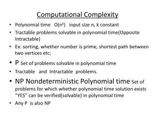
Useful notation Let f , g : D gR+ be two functions. We say that f is O(g) (and sometimeswrite f=O(g)) if there existconstantsα, β >0 such that f(x) αg(x)+β for all xD. If f= O(g)andg= O(f)we also say that f= Θ(g) (and of course g= Θ(f)). In this case, f and g have the samerate of growth.
Running time Let A be an algorithm which accepts inputs from a set X, and let f: DgR+. If there exist a constantα>0 such that A terminates its computation after at most αf(x)elementary steps (including arithmetical operations) for each input xX, then we say that A runs in O(f)time.We also say that therunning time (or thetime complexity)of A is O(f).
Input size The input size of an instance with rational data is the total number of bits needed for the binary representation.
Polynomial-time algorithm An algorithm with rational input is said to run in polynomial time if there is an integer k such that it runs in O(nk) time,where n is the input size, and all numbers in intermediate computations can be sorted with O(nk) bits. An algorithm with arbitrary input is said to run in strongly polynomial time if there is an integer k such that it runs in O(nk) time for any input consisting of n numbers and it runs in polynomial time for rational input. In the case k=1we have a linear-time algorithm.
Simple Reductions Between Scheduling Problems G R ○ X Q k O J P 2 3 4 F
Simple Reductions Between Goal Functions Σ wjTj Σ wjUj Σ wjCj ΣTj ΣUj ΣCj Lmax Cmax
General Property Lemma 4.0 If all rj= 0 and if the objective function is a regular function of the finishing times of the jobs, then only schedules without preemption and without idle time need to be considered. This follows from the fact that the optimal objective value does not improve if preemption is allowed.
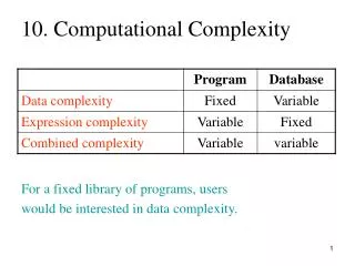
Proof of Lemma 4.0 Proof: Consider a schedule in which some job i is preempted • i isscheduled in [t1,t2[ and [t3,t4[ where t1< t2 < t3< t4 • i is neither scheduled in [t2,t3[ nor immediately before t1. If we reschedule so that the part of i occurring in [t1,t2[ is scheduled between t3– (t2 – t1) and t3, and so that anything scheduled between t2 and t3 is moved back units t2 – t1 of time, we eliminate this preemption of i without increasing the objective function. Continuing this process, we obtain an optimal solution for the preemptive problem where no preemption is necessary.
1|prec| fmax • Given are n jobs J1 ,..., Jn with precedence constraints to be processed on a single machine and monotone (nondecreasing) functions fj of the finish times Ci of jobs j = 1,..., n. • Task: Find a schedule that minimizes fmax = max j = 1,...,n fj(Ci).
Lawler’s Theorem Theorem 4.1 [Lawler 1973] The sequence constructed by the Lawler’s rule is optimal.
Proof of Theorem 4.1 1, 2,..., n is the sequence constructed by Lawler rule. σ: σ(1),..., σ(n) be an optimal sequence with σ(i) = i (i = n,...,r) and σ(r – 1) ≠ r – 1 where r is minimal. σ: r –1 k ● ● ● j r ● ● ● n tr r– 1 and j has no successor in the set {1,..., r– 1 } σ* is optimal σ*: k ● ● ● j r –1 r ● ● ● n
1| prec; rj | fmax i → j & ri+ pi> rj r’j =ri+ pi j → k r’k =ri+ pi+ pj j k i j k ri rj ri +pi rk t
Algorithms Modify rj Assume that the jobs are enumerated topologically (i.e. for all jobs i,j with i → j we have i < j). • Fori := 1 to n – 1 do • For j := i + 1 to n do • If i → j then rj:= max{rj, ri + pi} Now, we have rj > ri if i→j.
Block • Thus, if we schedule jobs according to nondecreasing release times such that the release times are respected, we always get a feasible schedule. Such a schedule may consists of several blocks. A block is a maximal set of jobs which are processed without any idle time between them. 1 2 idle time 3 4 5 idle time 6
Algorithm Blocks ({1, 2,..., n}) The following algorithm gives a precise description of blocks constructed in this way. We assume that all release times are modified and that the jobs are sorted according to these modified release times. Both algorithms are valid for preemptive and nonpreemptive schedules with jobs having arbitrary processing time.
1| prec; pmtn; rj| fmax Lemma 4.2 For problem 1| prec; pmtn; rj| fmaxthere exists an optimal schedule such that the intervals [sj,tj] (j = 1,..., k) constructed by Algorithms Blocks are completely occupied by jobs.
Proof of Lemma 4.2 σ: some optimal schedule [s, t]: the first idle interval inside some block interval [sj, tj] T: set of jobs starting later than time s in σ. σ: 1 2 idle time 3 4 5 idle time 6 sj–1 tj–1 sj s t tj i |ris & Ci(σ) > s OR r= min{rk | k T } > s Move job i into the idle interval so that either [s, t] is completely filled or job i finishes in [s, t] . Interval [s, r] must be an idle interval in the schedule created by Algorithms Blocks.
Conclusion • Due to Lemma 4.2 we may treat each block separately. The optimal solution value for the whole problem is given by the maximum of the solution values of all blocks.
Recursive rule A schedule is now constructed as follows. We solve the problem for the set of jobs B/{l}. the optimal solution of this problem again has a corresponding block structure. Similar to the proof of Lemma 4.2 we can show that job l can be scheduled in the idle periods of this block structure yielding a schedule with objective value of at the most which is the optimal value for B.
Example: f1=x2, f2=3x, f3=2x, f4=2x+5, f5=x+27. 1 2 3 4 5 t r5= 15 20 r1= 0 r2= 3 r3= 6 r4= 10
Example: f1=x2, f2=3x, f3=2x, f4=2x+5, f5=x+27. 1 2 3 4 5 t r5= 15 20 r1= 0 r2= 3 r3= 6 r4= 10 f1(20) = 400, f2(20) = 60, f3(20) = 40, f4(20) = 45, f5(20) = 47.
Example: f1=x2, f2=3x, f3=2x, f4=2x+5, f5=x+27. 1 2 3 4 5 t r5= 15 20 r1= 0 r2= 3 r3= 6 r4= 10 3 t 20 0 3 1 2 4 5 t r5= 15 20 r2= 3 r3= 6 r1= 0 r4= 10
Example: f1=x2, f2=3x, f3=2x, f4=2x+5, f5=x+27. 1 2 3 4 5 t r5= 15 20 r1= 0 r2= 3 r3= 6 r4= 10 1 2 4 5 t r5= 15 20 r1= 0 r2= 3 r3= 6 r4= 10 3 3 3 1 2 4 5 t r5= 15 20 r1= 0 r2= 3 r3= 6 r4= 10
Algorithm 1| prec; pmtn; rj| fmax • S := {1, 2,..., n}; • f*max := Decompose(S)
Procedure Decompose (S) • If S = then return –∞ ; • If S = {i} then return fi(ri + pi) else begin • Call Blocks (S); • f := –∞ ; • For all blocks B do • begin • Find l with fl(t(B)) = min{fj(t(B))| j B without succ. in B}; • h := Decompose(B\{l}); • f := max{f, h, fl(t(B))} • end • Return f end
Schedule • The procedure Decompose can be easily extended in such a way that the optimal schedule is calculated as well. We have to schedule job l in the idle periods of the schedule for B\{l}. This is done from left to right respecting rl. Due to the fact that all release dates are modified, job l will respect the precedence relations.
Running time • The complexity of the algorithm is O(n2). This can be seen as follows. If we exclude the recursive calls in Step 7, the number of steps for the Procedure Decompose is O(|S|). Thus, for the number f (n) of computational steps we have the recursion f (n) = cn + Σ f (ni) where ni is the number of jobs in the i-th block and Σni n.
1| prec; pj= 1; rj | fmax • If all data are integer, then all starting and finishing times of the blocks are also integer. Thus, if we apply the algorithm to a problem with unit processing times, no preemption is necessary. Therefore, our algorithm also solves problem 1| prec; pj= 1; rj | fmax.
Exercises • To explain why we can not use the proof of Lemma 4.2 in order to get the similar result for 1| prec; rj| fmaxproblem (without preemptions). • Analyze the running time of Algorithm 1| prec; pmtn; rj| fmax.
Exercise 4.1 • Find an optimal schedule for the following instance of 1| prec; pj= 1; rj | fmaxproblem. Precedence constraints: J1 → J7 and J3 → J5 .
Exercises • Prove Corollary 3.3 and Corollary 3.4. • Suppose f is strictly increasing, positive function. That is, f(x) > 0 for all x > 0 and f(x) > f(y) whenever x > y. Show that SPT (short processing time first) gives an optimal schedule for the problem 1||Σf(Cj).
Monge Array (3) • Corollary 3.4