Download
1 / 39
390 likes | 558 Views
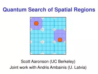
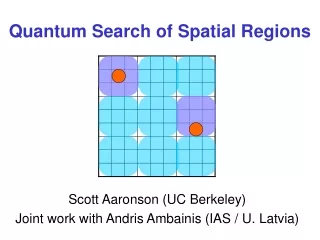
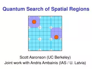
Quantum Search of Spatial Regions. Scott Aaronson (UC Berkeley) Joint work with Andris Ambainis (IAS / U. Latvia). Complexity Classes Not Needed For This Talk.

E N D
Quantum Search of Spatial Regions Scott Aaronson (UC Berkeley) Joint work with Andris Ambainis (IAS / U. Latvia)
Complexity Classes Not Needed For This Talk 0-1-NPC - #L - #L/poly - #P - #W[t] - +EXP - +L - +L/poly - +P - +SAC1 - AC - AC0 - AC0[m] - ACC0 - AH - AL - AM - AmpMP - AP - AP - APP - APX - AVBPP - AvE - AvP - AW[P] - AWPP - AW[SAT] - AW[*] - AW[t] - βP - BH - BPE - BPEE - BPHSPACE(f(n)) - BPL - BPPKT - BPP-OBDD - BPQP - BQNC - BQP-OBDD - k-BWBP - C=L - C=P - CFL - CLOG - CH - CkP - CNP - coAM - coC=P - coMA - coModkP - coNE - coNEXP - coNL - coNP - coNP/poly - coRE - coRNC - coRP - coUCC - CP - CSL - CZK - Δ2P - δ-BPP - δ-RP - DET - DisNP - DistNP - DP - E - EE - EEE - EEXP - EH - ELEMENTARY - ELkP - EPTAS - k-EQBP - EQP - EQTIME(f(n)) - ESPACE - EXP - EXPSPACE - Few - FewP - FNL - FNL/poly - FNP - FO(t(n)) - FOLL - FP - FPR - FPRAS - FPT - FPTnu - FPTsu - FPTAS - F-TAPE(f(n)) - F-TIME(f(n)) - GapL - GapP - GC(s(n),C) - GPCD(r(n),q(n)) - G[t] - HkP - HVSZK - IC[log,poly] - IP - L - LIN - LkP - LOGCFL - LogFew - LogFewNL - LOGNP - LOGSNP - L/poly - LWPP - MA - MAC0 - MA-E - MA-EXP - mAL - MaxNP - MaxPB - MaxSNP - MaxSNP0 - mcoNL - MinPB - MIP - MIPEXP - (Mk)P - mL - mNC1 - mNL - mNP - ModkL - ModkP - ModP - ModZkL - mP - MP - MPC - mP/poly - mTC0 - NC - NC0 - NC1 - NC2 - NE - NEE - NEEE - NEEXP - NEXP - NIQSZK - NISZK - NL - NLIN - NLOG - NL/poly - NPC - NPC - NPI - NP intersect coNP - (NP intersect coNP)/poly - NPMV - NPMV-sel - NPMVt - NPMVt-sel - NPO - NPOPB - NP/poly - (NP,P-samplable) - NPR - NPSPACE - NPSV - NPSV-sel - NPSVt - NPSVt-sel - NQP - NSPACE(f(n)) - NTIME(f(n)) - OCQ - OptP - PBP - k-PBP - PC - PCD(r(n),q(n)) - P-close - PCP(r(n),q(n)) - PEXP - PF - PFCHK(t(n)) - Φ2P - PhP - Π2P - PK - PKC - PL - PL1 - PLinfinity - PLF - PLL - P/log - PLS - PNP - PNP[k] - PNP[log] - P-OBDD - PODN - polyL - PP - PPA - PPAD - PPADS - P/poly - PPP - PPP - PR - PR - PrHSPACE(f(n)) - PromiseBPP - PromiseRP - PrSPACE(f(n)) - P-Sel - PSK - PSPACE - PT1 - PTAPE - PTAS - PT/WK(f(n),g(n)) - PZK - QAC0 - QAC0[m] - QACC0 - QAM - QCFL - QH - QIP - QIP(2) - QMA - QMA(2) - QMAM - QMIP - QMIPle - QMIPne - QNC0 - QNCf0 - QNC1 - QP - QSZK - R - RE - REG - RevSPACE(f(n)) - RHL - RL - RNC - RPP - RSPACE(f(n)) - S2P - SAC - SAC0 - SAC1 - SC - SEH - SFk - Σ2P - SKC - SL - SLICEWISE PSPACE - SNP - SO-E - SP - span-P - SPARSE - SPP - SUBEXP - symP - SZK - TALLY - TC0 - TFNP - Θ2P - TREE-REGULAR - UCC - UL - UL/poly - UP - US - VNCk - VNPk - VPk - VQPk - W[1] - W[P] - WPP - W[SAT] - W[*] - W[t] - W*[t] - XP - XPuniform - YACC - ZPE - ZPP - ZPTIME(f(n)) More at http://www.cs.berkeley.edu/~aaronson/zoo.html
Quantum Computing Model of computation based on our best-confirmed physical theory State of computer is superposition over strings: Most famous algorithm: Shor’s algorithm for factoring This talk: Grover’s algorithm for search
Grover’s Search Algorithm Unsorted database of n items Goal: Find one “marked” item • Classically, order n queries to database needed • Grover 1996: Quantum algorithm using order n queries • BBBV 1996: Grover’s algorithm is optimal
Grover Illustration Initial Superposition |000 |001 |010 |011 |100 |101
Grover Illustration Amplitude of Solution State Inverted |100 |000 |001 |010 |011 |101
Grover Illustration All Amplitudes Inverted About Mean |000 |001 |010 |011 |100 |101
BWAHAHA! Look who needs physics now! Grover’s Algorithm: Great for combinatorial search But can it help search a physical region?
Speed of light is finite Consider a quantum robot searching a 2D grid: n Robot Marked item n We need n Grover iterations, each of which takes n time, so we’re screwed! What even a dumb computer scientist knows: THE SPEED OF LIGHT IS FINITE
Talk Outline • The Physics of Databases • Algorithm for Space Search • Application: Disjointness Protocol • Open Problems
Trouble: Suppose our “hard disk” has mass density We saw Grover search of a 2D grid presented a problem… So why not pack data in 3 dimensions? Then the complexity would be n n1/3 = n5/6
Holographic principle Once radius exceeds Schwarzschild bound of (1/), hard disk collapses to form a black hole Makes things harder to retrieve… Actually worse—even a 2D hard disk would collapse once radius exceeds (1/)! 1D hard disk would not collapse… But we care about entropy, not mass A ball of radiation of radius r has energy (r) but entropy (r3/2)
Holographic principle Holographic Principle:A region of space can’t store more than 1.41069 bits per meter2 of surface area So Quantum Mechanics and General Relativity bothyield a n lower bound on search If space had d>3 dimensions, then relativity bound would be weaker: n1/(d-1) Is that bound achievable? Apparently not, since even stronger limit (Bekenstein’s) applies for weakly-gravitating systems
What We Will Achieve If n ~ rc bits are scattered in a 3D ball of radius r (where c3 and bits’ locations are known), search time is (n1/c+1/6) (up to polylog factor) For “radiation disk” (n ~ r3/2): (n5/6) = (r5/4) For n ~ r2 (saturating holographic bound): (n2/3) = (r4/3) To get O(n polylog n), bits would need to be concentrated on a 2D surface
Objections to the Model • Would need n parallel computing elements to maintain a quantum database • Response: Might have n “passive elements,” but many fewer “active elements” (i.e. robots), which we wish to place in superposition over locations • (2) Must consider effects of time dilation • Response: For upper bounds, will have in mind weakly-gravitating systems, for which time dilation is by at most a constant factor
Back to the Main Issue Classical search takes (n) time Quantum search takes (rn) (r = maximum radius of region) Can we do anything better? Benioff (2001): Guess we can’t…
Revenge of computer science • Idea: Recursively divide into sub-squares Using amplitude amplification techniques of BHMT’2002, we get: O(n log3n) for 2D grid O(n) for 3 and higher dimensions REVENGE OF COMPUTER SCIENCE • We can.
What’s the Model? • Undirected connected graph G=(V,E) • Bit xi at each vertex vi • Goal: Compute some Boolean f(x1…xn){0,1} • State can have arbitrary ancilla z: • Alternate query transforms • with ‘local’ unitaries • What does ‘local’ mean? Depends on your religion
Locality religions FARHIOLOGY H THERE IS ONLY THE HAMILTONIAN Defining Locality: 3 Choices (1) Unitary must be decomposable into commuting local operations, each acting on a single edge (2) Just don’t “send amplitude” between non-adjacent vertices: if (i,j)E then (3) Take U=eiH where H has eigenvalues of absolute value at most , and if (i,j)E then (1) (2),(3). Upper bounds will work for (1); lower bounds for (2),(3). Whether they’re equivalent is open
Amplitude AmplificationBrassard, Høyer, Mosca, Tapp 2002 • Generalization of Grover search • If a quantum algorithm has success probability , then by invoking it 2m+1 times (m=O(1/)), we can make the success probability
In More Detail: d3 • Assume there’s a unique marked item • Divide into n1/5 subcubes, each of size n4/5 • Algorithm A: • If n=1, check whether you’re at a marked item • Else pick a random subcube and run A on it • Repeat n1/11 times using amplitude amplification • Running time:
d3 (continued) • Success probability (unamplified): • With amplification: • (since is negligible) • Amplify whole algorithm n1/22 times to get
d=2 • Here diameter of grid (n) exactly matches time for Grover search • So we have to recurse more, breaking into squares of size n/log n • Running time suffers correspondingly: • (best we could get)
Multiple Marked Items • If exactly r marked items: • for d3. Basically optimal: • If at least r marked items, can use “doubling trick” of BBHT’98 to get same bound for d3. For d=2 we get
Search on Irregular Graphs • Our algorithm can be adapted to any graph with good expansion properties (not just hypercubes) • Say G is d-dimensional if for any v, number of vertices at distance r from v is (min{rd,n}) • Can search in time • Main idea: Build tree of subgraphs bottom-up
Bits Scattered on a Graph • If G is >2-dimensional, and has h possible marked items (whose locations are known), then • Intuitively: Worst case is when bits are scattered uniformly in G
Application: Disjointness • Problem: Alice has x1…xn{0,1}n, Bob has y1…yn They want to know if xiyi=1 for some i • How many qubits must they communicate? • Buhrman, Cleve, Wigderson 1998: • Høyer, de Wolf 2002: • Razborov 2002:
Disjointness in O(n) Communication B A State at any time: Communicating one of 6 directions takes only 3 qubits
Random walk Open Problem #1 Can a quantum walk search a 2D grid efficiently? (Maybe even n time instead of n log3n?) Promising numerical evidence (courtesy N. Shenvi)
Update (1 month ago) Childs, Farhi, Goldstone et al.: Rigorous proof that random walk searches 5-D hypercube in O(n) time, 4-D hypercube in O(n polylog n) time (or so they tell me)
Starfish n Open Problem #2 Here’s a graph of diameter n that takes (n3/4) time to search (by BBBV’96 hybrid argument): Does it also take (n3/4) time to decide if every row of a 2D grid has a marked item?
2D Turing machine Open Problem #3 Cosmological constant 10-122 > 0 (type-Ia supernova observations) Number of bits accessible to any one observer is at most 3/ (Bousso 2000, Lloyd 2002) How many of those ~10123 bits could a computer “use” before they recede past its horizon? Our result shows a quantum computer could search more of the bits than a classical one But what about using them as memory?
0 0 0 0 1 1 The Inflationary Turing Machine 1 1
0 0 0 0 1 1 The Inflationary Turing Machine 1 1
0 0 0 0 1 1 The Inflationary Turing Machine 1 1
0 0 0 0 1 1 The Inflationary Turing Machine 1 1
0 0 0 0 1 1 The Inflationary Turing Machine 1 1 At each time step t, a new tape square (initialized to 0) is created after square k/ - t for each integer k Toy model for > 0 spacetime
2D Turing machine Open Problem #3 (con’t) Consider a 2D Turing machine with O(n) time, a square worktape, and a separate input tape Is there anything it can do with an nn worktape that it can’t do with a nn worktape? What about a quantum TM? Related to Feige’s embedding problem: Given n checkers on an nn checkerboard, can we move them to an O(n)O(n) board so that no 2 checkers become farther apart in L1 distance?
Conclusions Not all strings have n bits • In a >0 spacetime, a quantum robot could search a larger region than a classical one (not assuming any time bound) • Physics is a good source of “pure” CS questions Quantum computing is just one example