Download
1 / 14
140 likes | 167 Views
Explore Scott Aaronson's research on Grover’s Search Algorithm in quantum search of spatial regions, optimization, limitations, applications, and recent progress. Dive into the implications of quantum mechanics and general relativity on search algorithms.

E N D
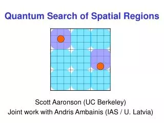
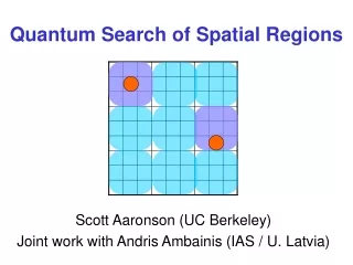
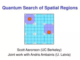
Quantum Search of Spatial Regions Scott Aaronson (UC Berkeley) Joint work with Andris Ambainis (U. Latvia)
Grover’s Search Algorithm Unsorted database of n items Goal: Find one “marked” item • Classically, (n) queries to database needed • Grover 1996: O(n) queries quantumly • BBBV 1996: Grover’s algorithm is optimal Great for combinatorial search—but can it help with a physical database?
Consider a quantum robot searching a 2D grid: n Robot Marked item n We need n Grover iterations, each of which takes n time, so we’re screwed! What even a dumb computer scientist knows: THE SPEED OF LIGHT IS FINITE
What’s the Model? • Undirected connected graph G=(V,E) • Bit xi at each vertex vi • Goal: Compute some Boolean f(x1…xn){0,1} • State can have arbitrary workspace z: • | = i,z |vi,z • Alternate query transforms |vi,z (-1)x(i) |vi,z • with ‘local’ unitaries U • What does ‘local’ mean? Depends on your religion
Defining Locality: 3 Choices (2) Zero pattern of U respects graph • Decomposability U is a product of commuting edgewise operations (3) Zero pattern of Hamiltonian H respects graph U = eiH H has bounded eigenvalues (1) (2),(3) Upper bounds work for (1) Lower bounds for (2),(3) Whether they’re equivalent is open
Trouble: Suppose our “hard disk” has mass density We saw Grover search of a 2D grid presented a problem… So why not pack data in 3 dimensions? Then the complexity would be n n1/3 = n5/6
Once radius exceeds Schwarzschild bound of (1/), database collapses to form a black hole Makes things harder to retrieve… Holographic Principle:Best one can do asymptotically is store data on a 2D surface, 1.41069 bits/meter2 So Quantum Mechanics and General Relativity bothyield a n lower bound on search But can we search a 2D region in less than n steps? Benioff (2001): Guess we can’t…
Revenge of computer science • Example: Take a classical subroutine that searches a square of size n in n stepsRun n copies in superposition and use Grover O(n3/4) (n time to move across grid is needed for subroutine anyway) By adding more levels of recursion, can make running time O(n1/2+) REVENGE OF COMPUTER SCIENCE • We can. Can we do better? Say n?
Amplitude AmplificationBrassard, Høyer, Mosca, Tapp 2002 Theorem: If a quantum algorithm has success probability p and returns a certificate, then by invoking it m times, m=O(1/p), we can amplify success probability to (1-m2p/3)m2p Diminishing returns Success Probability Better to keep prob low & amplify later # of Iterations
Algorithm for d3 Dimensions T(n) n1/11(T(n4/5)+O(n1/d)) = O(n5/11) P(n) (1-)n2/11n-1/5P(n4/5) = (n-1/11) (we show is negligible) Running Time: Success Prob: Amplify whole algorithm n1/22 times to get T(n) = O(n1/22n5/11) = O(n), P(n) = (1) • Assume there’s a unique marked item • Divide into n1/5 subcubes, each of size n4/5 • Algorithm A: • If n=1, check whether you’re at a marked item • Else pick a random subcube and run A on it • Amplify n1/11 times
Summary of Bounds When d=2, time for Grover search matches radius of grid An arbitrary graph is d-dimensional if for any vertex v, number of vertices at distance r from v is (min{rd,n}) When there are h possible marked items with known locations, the worst case is that they’re evenly scattered
Application: Disjointness • Problem: Alice has x1…xn{0,1}n, Bob has y1…yn They want to know if xiyi=1 for some i • How many qubits must they communicate? • Buhrman, Cleve, Wigderson 1998: O(n log n) • Høyer, de Wolf 2002: O(n clog*n) • Razborov 2002: (n)
Disjointness in O(n) Communication B A State at any time: i,z(A),z(B) |vi,zA |vi,zB Communicating one of 6 directions takes only 3 qubits
Recent Progress Childs-Goldstone: Spatial search by quantum walk O(n5/6) for d=3, O(n log n) for d=4, O(n) for d>4 Running time not competitive with ours in low dimensions, but less memory needed Ambainis-Kempe: Discrete walk with 2-bit coin O(n log n) for d=2, O(n) for d3 Connection to Dirac equation?