Download

1 / 22
250 likes | 552 Views
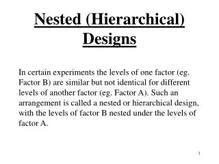
Hierarchical (nested) ANOVA. Hierarchical ANOVA. Hierarchical (nested) ANOVA. In some two-factor experiments the level of one factor , say B, is not “cross” or “cross classified” with the other factor, say A, but is “NESTED” with it. The levels of B are different for different levels of A.

E N D
Hierarchical ANOVA Hierarchical (nested) ANOVA • In some two-factor experiments the level of one factor , say B, is not “cross” or “cross classified” with the other factor, say A, but is “NESTED” with it. • The levels of B are different for different levels of A. • For example: 2 Areas (Study vs Control) • 4 sites per area, each with 5 replicates. • There is no link from any sites on one area to any sites on another area.
Hierarchical ANOVA Study Area (A) Control Area (B) S1(A) S2(A) S3(A) S4(A) S5(B) S6(B) S7(B) S8(B) X X X X X X X X X X X X X X X X X X X X X X X X X X X X X X X X X X X X X X X X X = replications Number of sites (S)/replications need not be equal with each sites. Analysis is carried out using a nested ANOVA not a two-way ANOVA. • That is, there are 8 sites, not 2.
Hierarchical ANOVA • A Nested design is not the same as a two-way ANOVA which is represented by: A1 A2 A3 B1 X X X X X X X X X X X X X X X B2 X X X X X X X X X X X X X X X B3 X X X X X X X X X X X X X X X Nested, or hierarchical designs are very common in environmental effects monitoring studies. There are several “Study” and several “Control” Areas.
Hierarchical ANOVA Objectives • The nested design allows us to test two things: (1) difference between “Study” and “Control” areas, and (2) the variability of the sites within areas. • If we fail to find a significant variability among the sites within areas, then a significant difference between areas would suggest that there is an environmental impact. • In other words, the variability is due to differences between areas and not to variability among the sites.
Hierarchical ANOVA • In this kind of situation, however, it is highly likely that we will find variability among the sites. • Even if it should be significant, however, we can still test to see whether the difference between the areas is significantly larger than the variability among the sites with areas.
Hierarchical ANOVA Statistical Model Yijk = m + ri + t(i)j + e(ij)k i indexes “A” (often called the “major factor”) (i)j indexes “B” within “A” (B is often called the “minor factor”) (ij)k indexes replication i = 1, 2, …, M j = 1, 2, …, m k = 1, 2, …, n
Hierarchical ANOVA Model (continue)
Hierarchical ANOVA Model (continue) Or, TSS = SSA + SS(A)B+ SSWerror = Degrees of freedom: M.m.n -1 = (M-1) + M(m-1) + Mm(n-1)
Hierarchical ANOVA Example M=3, m=4, n=3; 3 Areas, 4 sites within each area, 3 replications per site, total of (M.m.n = 36) data points M1 M2 M3Areas 1 23 45678 9101112 Sites 10 12 8 13 11 13 9 10 13 14 7 10 14 8 10 12 14 11 10 9 10 13 9 7 Repl. 9 10 12 11 8 9 8 8 16 12 5 4 11 10 10 12 11 11 9 9 13 13 7 7 10.75 10.0 10.0 10.25
Hierarchical ANOVA Example (continue) SSA = 4 x 3 [(10.75-10.25)2 + (10.0-10.25)2 + (10.0-10.25)2] = 12 (0.25 + 0.0625 + 0.625) = 4.5 SS(A)B = 3 [(11-10.75)2 + (10-10.75)2 + (10-10.75)2 + (12-10.75)2 + (11-10)2 + (11-10)2 + (9-10)2 + (9-10)2 + (13-10)2 + (13-10)2 + (7-10)2 + (7-10)2] = 3 (42.75) = 128.25 TSS = 240.75 SSWerror= 108.0
Hierarchical ANOVA ANOVA Table for Example Nested ANOVA: Observations versus Area, Sites Source DF SS(平方和) MS(方差) F P Area 2 4.50 2.25 0.158 0.856 Sites (A)B 9 128.25 14.25 3.167 0.012** Error 24 108.00 4.50 Total 35 240.75 What are the “proper” ratios? E(MSA) = s2 + V(A)B + VA E(MS(A)B)= s2 + V(A)B E(MSWerror) = s2 = MSA/MS(A)B = MS(A)B/MSWerror
Hierarchical ANOVA Summary • Nested designs are very common in environmental monitoring • It is a refinement of the one-way ANOVA • All assumptions of ANOVA hold: normality of residuals, constant variance, etc. • Can be easily computed using SAS, MINITAB, etc. • Need to be careful about the proper ratio of the Mean squares. • Always use graphical methods e.g. boxplots and normal plots as visual aids to aid analysis.
Hierarchical ANOVA Sample:Hierarchical (nested) ANOVA Length mosquito cage 58.5 1 1 59.5 1 1 77.8 2 1 80.9 2 1 84.0 3 1 83.6 3 1 70.1 4 1 68.3 4 1 69.8 1 2 69.8 1 2 56.0 2 2 54.5 2 2 50.7 3 2 49.3 3 2 63.8 4 2 65.8 4 2 56.6 1 3 57.5 1 3 77.8 2 3 79.2 2 3 69.9 3 3 69.2 3 3 62.1 4 3 64.5 4 3
Hierarchical ANOVA Length = β0 + βcage╳ cage +βmosquito(cage)╳ mosquito (cage) + error df?
Hierarchical ANOVA data anova6; input length mosquito cage;cards; 58.5 1 1 59.5 1 1 77.8 2 1 80.9 2 1 84.0 3 1 83.6 3 1 70.1 4 1 68.3 4 1 69.8 1 2 69.8 1 2 56.0 2 2 54.5 2 2 50.7 3 2 49.3 3 2 63.8 4 2 65.8 4 2 56.6 1 3 57.5 1 3 77.8 2 3 79.2 2 3 69.9 3 3 69.2 3 3 62.1 4 3 64.5 4 3 ; procglmdata=anova6; class cage mosquito; model length = cage mosquito(cage); testh=cage e=mosquito(cage); outputout = out1 r=res p=pred; procprintdata=out1;var res pred; procplotdata = out1;plot res*pred; procunivariatedata=out1 normalplot;var res; run;
Hierarchical ANOVA Class Levels Values mosquito 4 1 2 3 4 cage 3 1 2 3 Number of observations 24
Hierarchical ANOVA Sum of Source DF Squares Mean Square F Value Pr > F Model 11 2386.353333 216.941212 166.66 <.0001 Error 12 15.620000 1.301667 Corrected Total 23 2401.973333 Source DF Type I SS Mean Square F Value Pr > F cage 2 665.675833 332.837917 255.70 <.0001 mosquito(cage) 9 1720.677500 191.186389 146.88 <.0001 Tests of Hypotheses Using the MS for mosquito(cage) as an Error Term Source DF Type I SS Mean Square F Value Pr > F cage 2 665.675833 332.837917 1.74 0.2295
Hierarchical ANOVA res1 res
Hierarchical ANOVA res pred
Hierarchical ANOVA Tests for Normality Test --Statistic--- -----p Value------ Shapiro-Wilk W 0.978828 Pr < W 0.8733 Kolmogorov-Smirnov D 0.093842 Pr > D >0.1500 Cramer-von Mises W-Sq 0.038078 Pr > W-Sq >0.2500 Anderson-Darling A-Sq 0.22057 Pr > A-Sq >0.2500
Hierarchical ANOVA Two way ANOVA vs. nested ANOVA