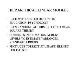
HIERARCHICAL LINEAR MODELS
HIERARCHICAL LINEAR MODELS. NESTED DESIGNS.

HIERARCHICAL LINEAR MODELS
E N D
Presentation Transcript
NESTED DESIGNS • A factor A is said to be nested in factor B if the levels of A are divided among the levels of B. This is given the notation A(B). We have encountered nesting before, since Subjects are typically nested in Treatment, S(T), in the randomized two group experiment.
ANOVA TABLE Note: no interactions can occur between nested factors
ESTIMATING VARIANCES 2C = (MSC – MSP )/p Conceptually this is = (2 +p2c - 2)/p
TESTING CONTRASTS • Thus, if one wanted to compare School 1 to School 2, the contrast would be C12 = [ Xschool 1 - Xschool 2 ] • Since the school mean is equal to overall mean + school 1 effect + error of school: • Xschool 1 = ...+ 1. + e1. ,
TESTING CONTRASTS • the variance of School 1 is • VAR(Xschool 1 ) = { 2 + 2S }/s • = { MS(P(C(S))) + [MS(S) - MS(C(S)]/cp} / s Then t = C12/{ 2[MS(P(C(S)))+[MS(S)-MS(C(S)]/cp]/s} which is t-distributed with 1, df= Satterthwaite approximation
Satterthwaite approximation df= { cpMS(P(C(S)))/s + [MS(S) - MS(C(S)]/s }2 {cpMS(P(C(S)))/s }2 + {[MS(S)}2 + {MS(C(S)]/s }2 (p-1)cs cp(s-1) p(c-1)
HLM - GLM differences • GLM uses incorrect error terms in HLM designs • Multiple comparisons using GLM estimates will be incorrect in many designs • HLM uses estimates of all variances associated with an effect to calculate error terms
Repeated Measures • Multiple measurements on the same individual • Time series • Identically scaled variables • Measurements on related individuals or units • Siblings (youngest to oldest among trios of brothers) • Spatially ordered observations along a dimension
WITHIN-GROUP DESIGNS Within group designs We encountered a repeated measures design in Chapter Six in the guise of the dependent t-test design. : _ _ t = x1. – x2. / sd where sd = [ ( s21 + s22 – 2 r12 s1s2 )/n ]1/2
WITHIN-GROUP DESIGNSMODEL • y ij = + i + j + eij • where y ij = score of person i at time j, • = mean of all persons over all occasions, • i = effect of person i, • j = effect of occasion j, • eij = error or unpredictable part of score.
EXPECTED MEAN SQUARESFOR WITHIN-GROUP DESIGN Source df Expected mean square 2 2 s s P P-1 + O p e 2 2 2 s s s O O-1 + + P t p t e 2 2 s s PO (P-1)(O-1) + t p e 2 s error 0 e Table 11.1: Expected mean square table for P x O design
ANOVA Table Source df SS MS F Within-subject 2 S Person P-1 O (y – y ) SS /(P-1) - i. .. P 2 S Occasion O-1 P (y – y ) SS /(O-1) MS /MS .j .. O O PO 2 SS P x O (P-1)(O-1) ( y – y ) SS /(P-1)(O-1) - ij .. PO error 0 0 - EXPECTED MEAN SQUARESFOR WITHIN-GROUP DESIGN
SPHERICITY ASSUMPTION ij = ij for all j, j (equal covariances) and ij = ij for all I and j (equal variances) By treating each occasion as a variable, we can represent this covariance matrix, called a compound symmetric matrix, as 11 12 13 … = 21 22 23 … 31 32 33 … . . with 12 =21 = 31 = 32
Testing Sphericity • GLM uses Huynh-Feldt or Greenhouse-Geisser corrections to the degrees of freedom as sphericity is violated • reduces degrees of freedom and power • HLM allows specifying the form of the covariance matrix • Compound symmetry (sphericity) • Autoregressive processes • Unstructured covariance (no limitations)
Between- and Within-group Designs BETWEEN SOURCE df SS MS F error term Treat 1 20 20 4.0 P(Treat) Person 18 90 5.0 - WITHIN Time 2 50 25 12.5 P(Treat) x Time Treat x Time 2 30 15 7.5 P(Treat) x Time P(Treat) x Time 36 72 2.0 -
Doubly Repeated (Time x Rep) Between and Within Design BETWEEN WITHIN Time Treatment Time x Treatment Person (Treatment) x Time Person (Treatment) Person (Treatment) x Rep Treatment x Rep x Time Person (Treatment) x Time x Rep Treatment x Rep Rep Time x Rep
HLM-GLM distinctions • HLM correctly estimates contrasts for any hierarchical between-factors • HLM correctly estimates all within-subject contrasts • GLM does not estimate within-subject contrasts correctly
The corrections to the F-test should be made given that the sphericity test was significant. For Greenhouse-Geisser, the df for the F-test are reduced to 1, N-1 or 1, 1658, so that the F-statistic is still significant at p < .001. For the Huynh and Feldt epsilon statistic, the degrees of freedom are adjusted by the amount .732: dfnumerator = 3 x .732 = 2.196; dfdenominator = 4974 x .732 = 3640.968. The fraction df can either be rounded down or a program, such as available in SAS, can provide the exact probability. For the df = 2,3640 the F-statistic is still significant. Kirk (1996) discussed in detail various adjustments and recommends one by Collier, Baker, Mandeville, and Hayes (1967), but the computation is cumbersome; HLM analyses compute it.