Fully Self-Consistent Modeling of Continental Thermal Structure
Our research aims to advance thermal modeling of continents by accounting for convecting mantle heat flux and chemical structures within lithosphere. Existing models lack this crucial element, leading to multiple plausible models due to decoupling of local heat sources and mantle heat flow. Our three-pronged approach focuses on understanding the dynamic interaction between mantle convection and continent structures. By addressing the influence of long-lived continental lithosphere thickness and chemical composition on heat flow, we seek to refine thermal models for continental regions. This work represents a significant step towards achieving more accurate and consistent continental thermal modeling.

Fully Self-Consistent Modeling of Continental Thermal Structure
E N D
Presentation Transcript
TOWARD THE FULLY SELF-CONSISTENT MODELING OF CONTINENTAL THERMAL STRUCTURE T L R d 0.000 0.018 0.036 0.076 Ra 2 T = surface temperature s 100 R R d d=0.009 theory 1 simulation d=0.018 6 8 9 10 10 10 T = lid base temperature T = base temperature T = avg internal temperature i L b d=0.036 K = fluid thermal conductivity K = lid thermal conductivity L F d=0.076 Nu 10 d=0.140 12 8 11 10 4 9 6 7 7 8 5 10 10 10 10 10 10 10 10 10 10 10 V T 1 10 10 12 Ra = 10 L = 0.2 d= 0.018 Ra = 10 L = 0.6 d= 0.018 9 10 11 10 10 10 10 Ra 50 theory 40 simulation d=0.009 30 % variation 3 7 10 10 10 7 10 10 10 10 10 T - T 3 5 L s K (1 - T ) L L 20 q = K = C convecting mantle L d 3 2 T (d - d ) Ra failed region - extension L failed region - compression local geotherm cold hot 10 d=0.018 0 Ra warm mantle viscosity = 10 Pa s 21 upper crust lower crust “subducting” lithosphere viscosity = 10 Pa s 25 cratonic root 0 70 L 0.2 0.4 0.6 0.8 d Ra 140 bulk mantle 210 0.018 theory 280 simulation 100 9 Ra = 10 70 70 70 d=0.018 d=0.076 140 140 140 7 0.076 Ra = 10 Nu 210 210 210 d=0.018 10 d=0.076 280 280 280 5 Ra = 10 d=0.018 d=0.076 0.018 1 0 0.2 0.4 0.6 0.8 1 Lid Extent 300 300 mean %var no lidlid lid 250 250 theory 125.1 23.0 7.1 0.076 sim t1 120.6 23.4 7.7 200 200 sim t2 115.3 23.5 7.0 mean %var no lidlid lid Surface Heat Flux 150 150 Surface Heat Flux theory 151.4 27.8 5.0 Lid Lid Lid 100 100 sim t1 153.6 28.1 5.2 sim t2 181.4 27.7 5.2 50 50 0 0.2 0.4 0.6 0.8 1 0 0.2 0.4 0.6 0.8 1 Length Length 2 2 2 mW/m mW/m mW/m A. Lenardic & C.M. Cooper - Rice University L.-N. Moresi & H. Muhlhaus - CSIRO OVERVIEW: The equilibrium thermal structure of continents depends on the distribution of heat producing elements within the continental lithosphere and on its thermal conductivity structure. It also depends on the amount of heat coming from the convecting mantle. The majority of continental thermal models to date have not treated convective mantle heat flux directly. Rather, they have been based on solving the one-dimensional heat conduction equation in a layered medium meant to represent the lithosphere. This approach treats mantle heat flow as a free lower thermal boundary condition that is applied to a lithospheric column. Although this approach has proved useful, particularly when additional data constraints on deep thermal structure such as xenoliths exist, it can often hit a fundamental impasse in that a variety of models with different proportions of internal heat sources and mantle heat flow can be consistent with heat flow observations [Rudnick et al., 1998]. The reason the standard thermal modeling approach hits this impasse is because it inherently assumes that the component of heat coming from the convecting mantle is decoupled from the local chemical structure of the continental lithosphere and the strength and distribution of heat sources within it. That is, within this type of modeling approach mantle heat flow can take on a wide range of values for the same distribution and strength of crustal heat sources and vice versa. This is why a variety of models can be made to match heat flow data. Local mantle heat flux must, however, depend on the chemical structure and the amount of heat produced within a continent in some, as yet, unknown way, as these factors influences the local surface conditions that the convecting mantle experiences. If the dependence of local mantle heat flux on the local structure of continental lithosphere and on the amount of heat produced within it could be determined, then the range of allowable thermal models for any continental region could be more tightly constrained. In the broadest sense, this is the goal of the work presented here. THREE PRONGED APPROACH: The key missing ingredient in thermal models of continental lithosphere to date is the convecting mantle. Few models, geared specifically at constraining the equilibrium thermal structure of continental lithosphere, have treated mantle convection and continental chemical structure in a self-consistent way. This means that the majority of continental thermal models have had to make some type of assumption about the dynamics of mantle convection. The degree to which any of the assumptions are dynamically self-consistent with the derived thermal structure of the lithosphere will remain difficult to evaluate until the full range of dynamic interaction between mantle convection and continents is physically understood. This is a big task so if you are expecting a complete answer from this poster prepare to be disappointed. To break the task up a bit and to allow for the development of physical insight we have focussed on certain specific aspects of the full problem. Prong 1: The first aspect relates to answering the question of how the thickness of long-lived continental lithosphere effects the amount of heat that flows into its base from the mantle. If continental lithosphere is chemically distinct, stable, and preserved at the Earth’s surface for times exceeding the lifetime of oceanic lithosphere then, in effect, it forms a conducting lid that bounds the convecting mantle and to explore its equilibrium thermal structure one must attack the coupled problem involving the interaction of convection and conduction. An idealized system that is useful for building some insight into this coupling is that of a convecting fluid layer overlain by a conducting lid. The section explores such a system. Although idealized, keep in mind that theories of mantle heat loss have not considered conjugate heat transfer issues directly which must be done to get at continental thermal structure. So best to start simple to build needed insight. Prong 2: The full lid stuff is overly idealized in many ways. One key way relates to the fact that continents have finite lateral extent. So the second specific aspect of the larger problem that we consider is how does the situation explored in the full lid section change when the continental analogs have a finite extent. Any issue tied to mantle heat partitioning between oceans at continents at present or over time is related, to some degree, to this question. From a pure fluid dynamics point of view, few theories exist for the case of thermal convection with imposed lateral asymmetry. Thus exploring the simple analog system of the section is of use in moving toward our Earth oriented goal and also from a fluid dynamic viewpoint (it may also relate to insulating your house properly). Prong 3: We now move to numerical simulations that allow for a lot of Earth pertinent stuff not present in the simple analog systems. A long-term goal is to have a heat flow scaling theory that can address situations of the complexity of the simulations. The partial lid scalings will help move us toward such a theory and the simulations will test it. For now, the simulations are presented on a stand alone basis. An interesting result is that local mantle heat flow into a continent decreases as internal crustal heat goes up. This shows the non seperability of the problem. One can not safely solve for continental thermal structure by considering a conduction solution with a lower boundary condition prescribed for mantle convection as convective flux depends on the structure of the conductive portion of the lithosphere. The simulations, & partial lid scalings, also show that local thermal structure depends on the % of continental to oceanic lithosphere. Thus, continental growth comes into play. By the way, an extended theory predicts the results rather well but more later after it’s fully tested ... D = system depth T s d = lid thickness Lid K L d T L K F D * T i * =active thermal boundary layer thickness Convecting Fluid * * key unknowns to be solved for T b MAIN ASSUMPTIONS: 1) System is bottom heated & tends toward thermal equilibrium so that a) heat flow into lid base equals heat flow out b) heat flow into fluid equals heat out of fluid 2) Nearly linear thermal gradient holds across lid and across active thermal boundary layer of fluid. 3) The local boundary layer Rayleigh number remains near a constant value [Howard, 1966] Express the Assumptions Symbolically, Do Some Algebra & We Get: scaling constant non-dimensional avg surface heat flux and non-dimensional lid conductivity non-dimensional avg lid base temperature Rayleigh # based on the full system temperature drop non-dimensional lid thickness The graphs to the left compare scaling predictions to numerical simulation results for the average surface heat flux (top graph) and surface heat flux variations (bottom graph) versus Rayleigh number & non-dimensional lid thickness. Thermal fields from simulations are show in the images above. This allows us to determine the effects of lid thickness and thermal conductivity on heat flow for a given Rayleigh number. The degree of lateral heat flux variations can also be solved for (see preprint). Geotherm Envelopes for Increasing Root Thickness Mean Craton Heat Fluxes for Increasing Upper Crustal Heat Concentration 0 125 250 375 500 0 400 800 1200 1600 80 moho FULL LID SCALINGS AND SIMPLE NUMERICAL SIMULATIONS: The goal here is simple: for a convecting fluid layer covered by a conducting lid, predict the system heat transfer properties as a function of lid thickness, lid conductivity, fluid properties, and the applied temperature drop across the system. This is a conjugated heat transfer problem in that the degree of convective vigor in the fluid depends on the lid base temperature which itself depends on the degree of convective heat loss and on the properties of the conducting lid. This makes things a bit different from the classic Rayleigh-Bernard case in which the temperature drop driving convection is not part of the solution itself. The few simple assumptions noted above make the problem not as nasty as it may seem. Of course we must convince ourselves that the assumptions, and the scaling relations they lead to, are valid. To do this we have compared the scaling predictions to the results of numerical simulations that solve the full conservation equations describing thermal convection below a conducting lid. The results are good enough to convince us that the assumptions and the scaling ideas that follow from them are not at all bad. This system is very idealized relative to the Earth but the ideas developed can serve as a springboard to more complex situations such as allowance for internal heating and for lids of finite extent. root base Surface Heat Flux depth (km) 51 mean surface heat flux = 53 mW/m 2 moho 22 80 root base depth (km) mean surface heat flux = 52 mW/m 2 L 34.5 Crustal Heat Flux d Lid moho Prong 1: ~ ~ root base T 11 i depth (km) mean surface heat flux = 51 mW/m 18 Convecting Fluid 2 moho The First Main Assumption is that the analogy above is valid. Thus, if we know something about the thermal resistance in the no-lid zone, which we can get from classic boundary layer theory, and in the lid zone, which we can get from our full lid scaling, then we can build a composite thermal resistance via the circuit analogy. Its not only a matter of resistance as we must also consider the driving voltage, err that is to say, temperature drop. This depends on the average internal temperature of the convecting fluid. The Second Main Assumption is that this value is the volume weighted avg of the internal temperature for the lid and no lid case. Pictorially it looks like this: Mantle Heat Flux 13.5 depth (km) root base mean surface heat flux = 46 mW/m 2 9 0 125 250 375 500 0 400 800 1200 1600 Upper Crust Heat Generation Rate Relative to that of the Bulk Mantle o Temperature ( K ) Prong 2: solve for internal temp in no lid & full lid case then average accounting for % covered by lid & % free Geotherms from the center of a continent at several times from models with varied root thickness. Mean heat fluxes and variations can be extracted from the envelopes so as to map the effects of root thickness on continental thermal structure. Mean heat fluxes from the center of a continent from models with varied crustal heat. Notice that local mantle heat flux goes down as crustal heat goes up showing that mantle heat flow is not decoupled from continental heat generation rate. The upper graph to the left compares scaling predictions to numerical simulation results for the average surface heat flux versus Rayleigh number, lid thickness, & lid extent. The lower graphs to the left compare scaling predictions and simulation results for heat flux profiles across the full system. Thermal fields from simulations are show in the images above. REASONABLY COMPLEX NUMERICAL SIMULATIONS: The model shown above has a chemically distinct continent residing within the upper thermal boundary layer of a convecting mantle. The modeling formulation allows for a layered continental crust with each layer having distinct heat production & thermal conductivity (lateral variations can also incorporated although this is not employed above). Chemically distinct continental roots of variable shape and heat production are also allowed for. The amount of heat that flows into a section of continental lithosphere within the model is determined by the dynamics of mantle convection and its interaction with a continent. A version of the CITCOM finite element code is used to solve model equation. Both continental and oceanic plates are incorporated within the simulation. The incorporation of plate-like behavior relies on allowing for the formation of localized shear zones that represent plate margins. This is accomplished through the use of a visco-plastic rheology akin to that used by Moresi & Solomatov [1998] but also allowing for strain dependent weakening along the plastic rheologic branch [Tackley, 1998]. Continental lithosphere is assumed to be stable by giving it a very high viscosity, which prevents distributed ductile deformation, and a very high yield stress, which prevents localized shear zone formation. This assumption allows the equilibrium thermal profile within a presently stable continental section to be determined. It is not meant to isolate the factors that lead to stability. The preliminary results above explore how variations in crustal heat generation and root thickness affect global system dynamics. The coupled nature of the system explored means that local continental thermal structure is inseparably linked to global dynamics and must be considered in this context. The final scaling expressions are a bit cumbersome but are fully given in the preprint available w/ the poster Prong 3: PARTIAL LID SCALINGS AND SIMPLE NUMERICAL SIMULATIONS: The goal is much as it was for the full lid except that there is an added parameter, lid extent. This introduces a lateral symmetry breaking to the system which adds a bit of complexity. Again, a few simple assumptions can make things tractable. The basic one is that the lid and no lid regions of the system run in parallel. The full lid scaling already made an indirect circuit analogy in that it considered heat transfer through the lid and through the active thermal boundary layer of the fluid to run in series. We now take that series circuit and connect it in parallel to the free lid zone, whose resistance can be gotten at through classic boundary layer theory. A final assumption is needed to determine the average internal temperature which, following the circuit analogy, is needed to determine the voltage (temperature) drop driving electrical current (heat) out of the system. We make the simplest possible assumption to get at this. As with the full lid case we have tested the scaling relations that result. The partial lid theory allows for more stringent testing as it makes predictions not only about system averaged heat transfer but also about the heat transfer properties in the lid and no lid zone, i.e., it makes global and local predictions. The top & bottom center graphs show that global & local predictions match simulation results rather well. The theory is easily extended to cover any number of lids with internal thickness variations above a convecting fluid - just add a more resistors to the circuit. This can move us further from the idealized and toward the Earth-like case where heat transfer depends on multiple continents, with internal structure, interacting with a convecting mantle.