Download
1 / 34
340 likes | 461 Views
This study explores advanced techniques for extracting 200 Hz information from 50 Hz data in geophysical contexts. We discuss the significance of resolution—differentiating between diffraction and specular resolution—and the implications it has for accurate imaging. Through field tests and theoretical analysis, we delve into concepts like Evanescence Resolution and the potential for superresolution under various conditions. Our findings highlight the challenge of separating scattered fields and the importance of signal-to-noise ratios, thereby informing future applications in subsurface imaging and anomaly detection.

E N D
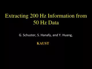
Extracting 200 Hz Information from 50 Hz Data G. Schuster, S. Hanafy, and Y. Huang, KAUST Sinc function Spiking function Rayleigh Resolution Profile Superresolution Profile
Outline • Motivation: Why Resolution Matters • Diffraction vs Specular Resolution: Example • Evanescence Resolution • Field Test • Conclusions
Resolution Dx~l/2 L Z Depth Δx Rayleigh Resolution: Δx KAUST yacht Abbe Resolution: Super Resolution?: Dx = Dx = Dx << lz l l 2 2 4L
Geophysical Resolution 0 km 3 km ? (Jianhua Yu) 0 km 7 km 0 km 7 km
Transmission+ReflectionWavepaths (Woodward, 1992) FWI rabbit ears d RTM smile Z RTM Resolution: Dx=Rayleigh, Dz=l/4 FWI Resolution: ? X
Transmission+ReflectionWavepaths (Woodward, 1992) FWI rabbit ears d Z FWI Resolution: X FWI Resolution: Dx= 2ld (Williamson, 1991)
Transmission+ReflectionWavepaths (Woodward, 1992) Diff. FWI Resolution: Dxdiff= ld FWI rabbit ears d 3 FWI Resolution: Benefit: Diffractions transform SSPXwellor VSP Data Liability: SNRdiff << SNRspec X FWI Resolution: Dx= 2ld (Williamson, 1991) Dx =2 Dxdiff
Summary Diff. FWI Resolution: Dxdiff= ldvsSpecular FWI Resolution: Dx = Benefit: Diffractions transform SSPXwellor VSP Data Liability: SNRdiff << SNRspec FWI rabbit ears 3
Outline • Motivation: Why Resolution Matters • Diffraction vs Specular Resolution: Example • Evanescence Resolution • Field Test • Conclusions
Diffraction Waveform Modeling 0 time (s) Born Modeling 4.0 Distance (km) 0 3.8 Scattered CSG Velocity 0 Depth (km) 1.2 Reflectivity 0 Depth (km) 1.2 0 Distance (km) 3.8
Diffraction Waveform Inversion True Velocity 0 Depth (km) 1.2 0 Distance (km) 3.8 Initial Velocity Inverted Velocity 0 0 Depth (km) Depth (km) 1.2 1.2 Estimated Reflectivity 0 Depth (km) 1.2 0 Distance (km) 3.8
Outline • Motivation: Why Resolution Matters • Diffraction vs Specular Resolution: Example • Evanescence Resolution • Field Test • Conclusions
Far-field Propagation l-limited Resolution eiwtxg G(g|x)= r Mig(z) l Time
Near-field Propagation l/20 Resolution eiwtxg G(g|x)= r r Evanescent energy Mig(z) Mig(z) Note: Time delay unable to distinguish 2 scatterers, but near-field amplitude changes can: Dx=l/20 l Time
Near-field Propagation l/20 Resolution eiwtxg G(g|x)= r r Evanescent energy Mig(z) Note: Time delay unable to distinguish 2 scatterers, but near-field amplitude changes can: Dx=l/20 If source is in farfield of scatterers & geophones in nearfield, superresolution possible l Time
Summary 1. Near-field Propagation l/20 Resolution Mig(z) If source is in farfield of scatterers & geophones in nearfield, superresolution possible reciprocity If source is in nearfield of scatterers & geophones in farfield, superresolution possible l Time
Summary 1. Near-field Propagation l/20 Resolution CRG Mig(z) If source is in farfield of scatterers & geophones in nearfield, superresolution possible reciprocity If source is in nearfield of scatterers & geophones in farfield, superresolution possible l Time
Outline • Motivation: Why Resolution Matters • Diffraction vs Specular Resolution: Example • Evanescence Resolution • Field Test • Conclusions
Dx ~ Dx ~ 0.1 0.01 0.7 Dx ~ Near-Field Scatterer Images
D z ~ 0.1 25 Near-Field Scatterers Image
25 Near-Field Scatterers Image Migration image at superresolution
Elastic Tunnel Test: 6 Near-Field Scatterers S wave P wave Vp=1.5 km/s Vs=0.75 km/s 40 m Vp=3.0 km/s Vs=1.5 km/s 100 m
Elastic Tunnel Test: 6 Near-Field Scatterers S wave P wave Vp=1.5 km/s Vs=0.75 km/s No scatterer data scattered data 40 m Vp=3.0 km/s Vs=1.5 km/s 100 m
Outline • Motivation: Why Resolution Matters • Diffraction vs Specular Resolution: Example • Evanescence Resolution • Field Test • Conclusions
Experimental Setup (Not to Scale) Superresolution Test Goal: Test superresolution imaging by seismic experiment Experiment: Data with and without a scatterer l=1.6 m
Experimental Setup (Not to Scale) Superresolution Test Goal: Test superresolution imaging by seismic experiment Experiment: Data with and without a scatterer l=1.6 m 0.2 m 0.6 m
l/4 Resolution (110 Hz) 0.5 m w/o scatterer with scatterer l/8 Resolution (55 Hz) Theory l with scatterer 0.5 m 220 Hz information from 55 Hz data
Summary Diff. FWI Resolution: Dxdiff= ldvsSpecular FWI Resolution: Dx = • Workflow • 1. Collect Shot gathers G(g|s ), separate scattered field • 2. m(s’) = S G(g,t|s’)* G(g,t|s ) • 3. TRM profiles • Synthetic Results Dx~l/10 • Limitations • Either src or rec in nearfield of subwavelength scatterer • Scattered field separated from specular fields is Big Challenge
Possible Applications SSP: Detect local anomalies, faults, and scatterer points around surface VSP: Find local anomalies, faults, and scatterer points around boreholes in VSP data Farfield? Ground Borehole
Earthquakes along a Fault Detect Fault Roughness Subduction zone TRM Profile
Earthquakes US Array Detect Near Surface Subduction zone TRM Profile