Download
1 / 16
160 likes | 183 Views
Explore the effects of climate change on air quality and regional climate, including the interaction of aerosols with climate and ozone pollution trends in the US. Research conducted at Harvard University sheds light on the connection between cyclones, emissions, and pollution episodes. Discover how changes in aerosol concentrations impact regional climate and surface temperatures. This study provides insights into the complex interplay between atmospheric factors and environmental outcomes.

E N D
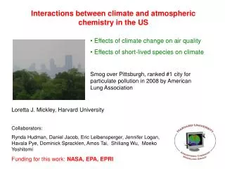
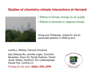
Studies of chemistry-climate interactions at Harvard • Effects of climate change on air quality • Effects of aerosols on regional climate Smog over Pittsburgh, ranked #1 city for particulate pollution in 2008 by ALA Loretta J. Mickley, Harvard University also Shiliang Wu, Jennifer Logan, Dominick Spracklen, Amos Tai, Rynda Hudman, Daniel Jacob, Moeko Yoshitomi, Eric Leibensperger, Havala Pye, Cynthia Lin Funding for this work: NASA, EPA, EPRI
Number of summer days with ozone exceedances, mean over sites in Northeast Northeast Probability of ozone exceedance vs. daily max. temperature • Curves include effects of • Biogenic emissions • Stagnation • Clear skies Probability Days 1988, hottest on record Southeast Los Angeles Temperature (K) I. Effects of climate change on air quality Weather plays a large role in ozone air quality. The total derivative d[O3]/dT is the sum of partial derivatives (dO3/dxi)(dxi/dT). x = ensemble of ozone forcing variables that are temperature-related. Lin et al., 2001
Cyclones crossing southern Canada affect ozone air quality in Eastern US. cold front L EPA ozone levels • Stalled high pressure system associated with: • increased biogenic emissions • clear skies • weak winds • high temperatures. cold front L 3 days later Cold front pushes smog poleward and aloft on a warm conveyor belt. Hazardous levels of ozone
Is there a connection between summertime cyclone frequency and the number of ozone episodes? Correlation of 1980-2006 JJA ozone exceedances with storm tracks Sample summertime storm tracks, 1979-81 weak correlation Strong anti-correlation NCEP/NCAR reanalysis • Frequentcyclones plus associated cold fronts mean fewer ozone episodes. • Fewer cyclones mean more persistent stagnation and more intense pollution. 6
0.14 a-1 0.16 a-1 1950-2000 observed trend in cyclone frequency matches that in climate model with increasing greenhouse gases. 1950-2006 trend in JJA cyclones in S. Canada Trend in cyclones appears due in part to weakened meridional temperature gradients, reduction of baroclinicity over midlatitudes. What does this trend mean for ozone pollution in US? Mickley et al., 2004; Leibensperger et al., 2008
Trend in emissions and trend in cyclones have competing effects on surface ozone. Cyclones: less frequent cyclones means longer pollution episodes Emissions: reduced emissions means fewer episodes. 1980-2006 trends cyclones NE ozone episodes Decline in emissions of ozone precursors from mobile sources, Parrish 2006. Mickley et al., 2004; Leibensperger et al., 2008
Ozone pollution days in the Northeast US Decline in mid-latitude cyclone number over mid-latitudes leads to more persistent stagnation episodes, more ozone. If cyclone frequency had remained constant, we calculate zero episodes over Northeast. Trend in pollution days due to decline in cyclone frequency days yr-1 days yr-1 Trend in pollution days due to decline in emissions days yr-1
II. Effects of aerosols on regional climate Present-day radiative forcing due to aerosols over the eastern US is comparable in magnitude, but opposite in sign, to global forcing due to CO2. Globally averaged radiative forcing due to CO2 is +1.7 Wm-2. warming Over the eastern US, radiative forcing due to sulfate aerosols is -2 Wm-2. cooling IPCC, 2007; Liao et al. , 2004
Is the climate response to changing aerosols collocated with regions of radiative forcing? Recent US Climate Change report says NO: Trends in short-lived species (such as aerosols) affect global, but not regional, climate. “Regional emissions control strategies for short-lived pollutants will . . . have global impacts on climate.” – U.S. Climate Change Science Program, Synthesis and Assessment Product 3.2 Harvard’s work to date says YES: Removal of the aerosol burden over the eastern US will lead to regional warming, in a way that the US Climate Change report would not have recognized. Calculated present-day aerosol optical depths
What is the influence of changing aerosol on regional climate? In pilot study, we zero out aerosol optical depths over US. GISS GCM For pilot study, 2 scenarios were simulated: Control: aerosol optical depths fixed at 1990s levels. Sensitivity: U.S. aerosol optical depths set to zero (providing a radiative forcing of about +2 W m-2 locally over the US); elsewhere, same as in control simulation. Each scenario includes an ensemble of 3 simulations.
Removal of anthropogenic aerosols over US leads to a 0.5-1o C warming in annual mean surface temperature. Additional warming due to zeroing of aerosols over the US. Warming due to 2010-2025 trend in greenhouse gases. Annual mean surface temperature change in Control. Mean 2010-2025 temperature difference: No-US-aerosol case – Control White areas signify no significant difference. Results from an ensemble of 3 for each case. Mickley et al., ms.
No-US-aerosols case Temperature (oC) Control, with US aerosols The regional surface temperature response to aerosol removal appears to persist for many decades in the model. Annual mean temperature trends over Eastern US Annual temperature difference between the two cases stays about constant, but in fact the annual mean hides seasonal differences. Mickley et al., ms
Additional warming due to aerosol removal over Eastern US fall winter spring Temperature (oC) summer The regional surface temperature response to aerosol removal varies according to season. 9-year running means. Stars indicate a significance difference between no-US-aerosols case and control : Winter: Temperature response is initially very strong, then dies off. Spring and Fall: Temperature response kicks in around 2030. Summer: Moderate temperature response. Mickley et al., ms
Additional warming due to aerosol removal over Eastern US fall winter spring Temperature (oC) summer Working hypothesis for time-dependent responses, varying by season. • Initial temperature response is strongest in winter. In the other seasons, excess surface heat can be more easily carried off through convection. • Rise in greenhouse gases increases stability of atmosphere, inhibits ventilation of warm surface air. Eventually surface warming in the no-US-aerosol case shows up in spring and fall. • In fall-winter-spring, the warming due to greenhouse gases eventually swamps the warming due to aerosol removal. Mickley et al., ms
Next steps: Perform more realistic simulation of changing aerosol optical depths over the US, together with sensitivity studies. • We use historical/projected emissions of SO2, NOx, BC, and OC to quantify the climatic role of US aerosols in the past and future. 1950-2050 Control simulation (EDGAR/Tami Bond historical emissions and A1B; includes rising U.S. aerosol sources until 1980 and subsequent decline) Sensitivity simulations: • 1950-2050 No US aerosols. Quantifies the past effect of U.S. anthropogenic sources on regional climate. • 2010-2050 Constant US emissions Quantifies the warming effect from the projected decrease in U.S. emissions. GEOS-Chem chemistry transport model aerosol concentrations Calculation of cloud droplet number concentrations aerosol indirect effect GISS GCM IIIclimate model Climate response to aerosol trends over the US
Calculated trend in surface sulfate concentrations, 1950- 2001. Sequence shows increasing sulfate from 1950-1980, followed by a decline in recent years. We will test the climate effects of this and other aerosol trends in the GISS climate model. 1950 1960 1970 1980 Comparison to observed sulfate concentrations shows good agreement. 1990 2001