Download
1 / 54
540 likes | 563 Views
Explore the basic principles of interferometry from historic experiments to modern applications, including coherence measurement, signal detection, and effects of Earth's atmosphere.

E N D
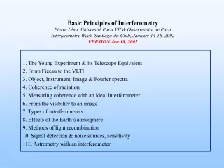
Basic Principles of InterferometryPierre Léna, Université Paris VII & Observatoire de ParisInterferometry Week, Santiago-du-Chili, January 14-16, 2002VERSION Jan.18, 2002 1. The Young Experiment & its Telescope Equivalent 2. From Fizeau to the VLTI 3. Object, Instrument, Image & Fourier spectra 4. Coherence of radiation 5. Measuring coherence with an ideal interferometer 6. From the visibility to an image 7. Types of interferometers 8. Effects of the Earth’s atmosphere 9. Methods of light recombination 10. Signal detection & noise sources, sensitivity 11. Astrometry with an interferometer
1. The Thomas Young Experiment • A founding experiment • Fringes & spatial structure of the source • The Telescope Equivalent
Reference : Glindeman, A., VLTI tutorial http://www.eso.org/projects/vlti/general/tutorial_introduction_to_stellar_interf.pdf
The Golden Rules of Interferometry • Relative modulation amplitude V (from 1 to 0) of the fringe pattern is related to the source angular size (a). • For a given source angular size, modulation amplitude decreases when separation of holes (B) increases. • For wavelength l, modulation becomes sensitive to size when a >≈ l /B
Wavelength l V.L.T. Baseline B
2. From Fizeau to the VLTI • 1802 Fringes and nature of light Thomas Young, Londres • 1868 Concept of interferometry with pupil mask Hippolyte Fizeau, Paris • 1872 Upper limit (0.158”) of stellar diameter Edouard Stephan, Marseille • 1921 First stellar diameter measurement Albert Michelson, Pasadena • 1950 First radio-interfometer Martin Ryle, Cambridge • 1956 First intensity interferometer (visible) R. Hanbury-Brown & R. Twiss • 1970 Speckle interferometry (visible) Antoine Labeyrie, Paris • 1972 First heterodyne fringes (10 m) Jean Gay & Alain Journet, Grasse • 1973 Deconvolution algorithm Leon Lucy • 1975 Triple correlation (visible) Gerd Weigelt, Nuremberg • 1976 Coupling two independent telescopes Antoine Labeyrie, Paris • 1987 Decision of VLT Interferometer Observatoire Européen Austral • 1989 First adaptive optics image (2.2 m) Gérard Rousset et al, Paris & ESO • 1996 First interferometric image (visible) James Baldwin, Cambridge • 2001 VLTI & Keck Interferometer first light C. Paranal, Chili & Mauna Kea • 2001 Adaptive optics on VLT (NAOS) Cerro Paranal, Chili
Albert Michelson’s Interferometric set-up, Mt. Wilson, Calif. 1920
Reference : Glindeman, A., VLTI tutorial http://www.eso.org/projects/vlti/general/ tutorial_introduction_to_stellar_interf.pdf
Antennas or telescopes ? Cambridge (UK) 1957, l = 1.7 m From Ryle’s Nobel Prize lecture, 1974
The first Labeyrie interferometer (1975-1980) Fringes on Vega at l = 550 nm
Three methods to achieve coherent combination of light : • change the frequency of light at each telescope, • carry to the common focus an Intermediate Frequency (IF) Signal, & combine all these signals (fringes) • : heterodyne interferometer (l from10 mm to mm-cm…) • receive the light at each telescope on a quantum detector • & correlate the photo-currents • : intensity interferometer (visible l) • Carry the light from each telescope to a common focus • & combine coherently, then detect interferometric signal (fringes), • : direct interferometer (optical l)
The Narrabri (Australia) Intensity Interferometer, constructed after the initial success of Hanbury-Brown & Twiss correlation on Sirius at visible wavelengths Nature (1956), 177, 27-29
2. From Fizeau to the VLTI • 1802 Fringes and nature of light Thomas Young, Londres • 1868 Concept of interferometry with pupil mask Hippolyte Fizeau, Paris • 1872 Upper limit (0.158”) of stellar diameter Edouard Stephan, Marseille • 1921 First stellar diameter measurement Albert Michelson, Pasadena • 1950 First radio-interfometer Martin Ryle, Cambridge • 1956 First intensity interferometer (visible) R. Hanbury-Brown & R. Twiss • 1970 Speckle interferometry (visible) Antoine Labeyrie, Paris • 1972 First heterodyne fringes (10 m) Jean Gay & Alain Journet, Grasse • 1973 Deconvolution algorithm Leon Lucy • 1975 Triple correlation (visible) Gerd Weigelt, Nuremberg • 1976 Coupling two independent telescopes Antoine Labeyrie, Paris • 1987 Decision of VLT Interferometer Observatoire Européen Austral • 1989 First adaptive optics image (2.2 m) Gérard Rousset et al, Paris & ESO • 1996 First interferometric image (visible) James Baldwin, Cambridge • 2001 VLTI & Keck Interferometer first light C. Paranal, Chili & Mauna Kea • 2001 Adaptive optics on VLT (NAOS) Cerro Paranal, Chili
3. Object, Instrument, Image & Fourier spectra • Object, instrument, image • Intensity (irradiance) in object/image and its spatial spectrum • Instrument as a spatial filter • Modulation Transfer Function (MTF) • Point Spread Function (PSF) • Isoplanatism • Degraded MTFs : aberrations, atmosphere
4. Coherence of radiation • The field radiation(r,t) and the source characteristics • Temporal coherence • Spatial coherence • Spatio-temporal coherence12() • Quasi-monochromatic case • Coherence over an illuminated surface : the Zernike-van Cittert theorem • Area of coherenceAc , étendueAc = l2, volume of coherence • Beam transport & coherence
5. Measuring coherence with an ideal interferometer • Principles of coherence (correlation) measurement • Fringes, complex visibility & source spatial spectrum • Some simple sources - point-like - uniform disk - binary star • Wavefront structure - loss of coherence : diffraction, scattering, atmospheric propagation - corrugation of amplitude and/or phase of visibility
Measuring spatial coherence : visibility amplitudes in optical interferometry Uniform disc star (Perrin,G. et al) From A. Glindeman’s VLTI tutorial
Chromatic dependence of spatial coherence The star g Cass M=16 Msun, R=6Rsun, D=100 pc GI2T Interferometer, Calern, France - Mourard et al., 1999
6. From the visibility to an image • Multiple baselines & synthetized pupil • The Single Telescope/Antenna MTF (Primary Beam) • The Interferometer MTF (Dirty Beam) • From Fourier space (visibilities) to image space : (N -> N) • Filling holes of the MTF : deconvolution techniques (« cleaning ») • Restoring a good PSF : the densified pupil
Aperture synthesis 1. Object is the Fourier transform of g(B/l) 2. g(B/l) is measured on a limited support -> Frequency cut-off 3. g(B/l) is measured on a sparse domain -> irregular PSF (Dirty beam) B Image plane (q) Fourier plane (u,v) N x N requires N x N
(VLTI) From A. Glindeman, VLTI tutorial
An example of Interferometer Point Spread Function (or Dirty Beam) The PSF of the ‘OHANA array (7 télescopes, source at zenith) 0.25 mas @ l =1 mm This would be the image of a point source. Cleaning the image of an extended object can be done with different techniques of deconvolution.
Etoile Wolf-Rayet WR 104 Peter Tuthill, Telescope Keck, 2000
VLTI OHANA interferometer on Mauna Kea
7. Types of interferometers • MTF of a real interferometer • The Fizeau recombination (optical) • The classical Michelson recombination (optical) • The Heterodyne recombination (radio) • Delay lines, : coherencing, cophasing, fringe tracking : optical & radio • Field-of-view of an interferometer : optical & radio • Polarisation effects • The densified pupil Michelson recombination LBT
A Fizeau interferometer : The Large Binocular Telescope (2 x 8.4 m), Mt Graham, Arizona Interferometric field-of-view = 1 arcmin (to compare with VLTI : 2 arcsec) Orion proplyds, HST 23 m 6 arcsec
coherencing cophasing wavetrain from telescope 1 wavetrain from telescope 2 zero OPD temporal coherence length ctc • Steps with metrology :` • Coherencing : find some fringes • Cophasing : adjust OPD=0 from star to fringe center through 1 & 2 • Fringe tracking : maintain OPD=0 with delay line (compensating for • Diurnal, atmospheric or instrument instant delays.
8. Effects of the Earth’s atmosphere • Overview on atmospheric coherence loss • Parameters :ro(o(, o (, Lo, lo • Adaptive optics, principle - Zernike polynomials description of wavefront - Strehl ratioS • Effects on interferometric observables ` - speckled fringes and visibility degradation - piston noise • Closure phase • Going to space !
IDEAL REEL Gerd Weigelt, Bonn
Loss of coherence (wavefront aberrations) on a single telescope : effect on fringes Telescope 1 + Telescope 2 (A. Glindeman, VLTI Tutorial)
Loss of coherence (differential piston) between 2 telescopes : effect on fringes Atmospheric Piston at 2.2 mm VLTI-UT1 & UT3 - Oct.2001 on Achernar
OPD=0 Star 2 is the bright object for piston tracking Star 1 is the faint object to be measured Star 2 Star 1 Piston tracking with reference
Summary of atmospheric effects on interferometric observations • adaptive optics on individual telescopes is needed. • But Strehl S <1 leads to visibility amplitude loss and visibility noise, • limiting accuracy. • piston noise between telescopes can not be compensated. • Limits exposure time, hence restricts observation to «bright» • objects & adds noise onto visibility amplitude measurement. • if differential piston is tracked on a «bright» source, long time • integration can be achieved to determine V of a «faint» source, • but atmosphere imposes a proximity(<≈ 1 arcmin). • differential piston makes absolute phase measurement of the • complex visibility impossible. Closure phase partially solves this. • absolute phase of source can yet be measured, if a known • (e.g. pointlike : star, quasar) phase calibrator lies close enough.
9. Methods of light recombination • Internal metrology in an interferometer • Image plane recombination - dispersed fringes & spectral analysis - pupil reconfiguration (Ntélescopes > 2) • Pupil plane recombination - Double Fourier spectral analysis • Integrated optics recombiners • Dual-beam (dual-feed) operation The VLTI Central Laboratory
10. Signal detection & noise sources, sensitivity • From measured to real visibility : calibration • Expression of the interferometric signal : amplitude & phase • Noise sources - signal photon noise (0.3 - 1mm) - detector read-out noise (1 to 2.5mm) - background (thermal) noise (2.5mm -> radio) - atmospheric noises (piston, scintillation) : alll • Sensitivity & accuracy
The interferometric signal (optical) • Complex visibility V exp(if) V Measuring (unwrapped) f needs a reference Telescope reference Another nearby object (star) Same object at different l