Process Dynamics of Input/Output Models: Numerical Approaches and Flow Diagram Analysis
This chapter explores essential concepts of process dynamics, focusing on input-output transfer functions in steady and unsteady states. It presents flow diagrams essential for understanding dynamic systems, numerical solving methods including finite difference, finite element, and finite volume methods, along with analytical Laplace solutions. Specific cases, such as concentration and level changes in a tank, are modeled and solved using Excel. Further homework tasks allow practical application of dynamic simulations, enhancing understanding of flow and concentration changes in process systems.

Process Dynamics of Input/Output Models: Numerical Approaches and Flow Diagram Analysis
E N D
Presentation Transcript
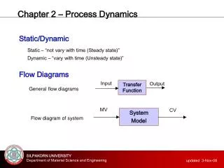
Chapter 2 – Process Dynamics Input Output Transfer Function MV CV System Model Static/Dynamic Static– “not vary with time (Steady state)” Dynamic– “vary with time (Unsteady state)” Flow Diagrams General flow diagrams Flowdiagram of system
Chapter 2 – Process Dynamics Part A: Numerical Solving - Finite difference method - Finite element method (FEM) - Finite volume method (FVM) Part B: Laplace Solving (analytical method)
Chapter 2 – Process Dynamics D Fin CA,in MV CV System Model CA h CA,in CA in Tank Fout CA,out Part A: Numerical Solving Case A: Conc. of A in tank (modelling) Flow Diagrams CA,out = CA
Chapter 2 – Process Dynamics Case A: Conc. of A in tank (modelling) Mass Flow Balance {rate of accummulation} = {rate of input} – {rate of output} + {rate of generation} – {rate of consumption}
Chapter 2 – Process Dynamics Case A: Conc. of A in tank (numerical) Finite Difference Numerical Solving
Chapter 2 – Process Dynamics Case A: Conc. of A in tank (on EXCEL) Numerical Solving
Chapter 2 – Process Dynamics Case A: Conc. of A in tank (on EXCEL) Numerical Solving
Chapter 2 – Process Dynamics D Fin CA,in MV CV System Model CA h Fin Level in Tank Fin CA,out Part A: Numerical Solving Case B: Level in tank (modelling) Flow Diagrams h orFout CA,out
Chapter 2 – Process Dynamics Case B: Level in tank (modelling) Mass Flow Balance {rate of accummulation} = {rate of input} – {rate of output} + {rate of generation} – {rate of consumption}
Chapter 2 – Process Dynamics Case B: Level in tank (modelling) Additional equation d = dia. of pipe
Chapter 2 – Process Dynamics Case B: Level in tank (Excel) Numerical Solving
Chapter 2 – Process Dynamics Case B: Level in tank (Excel) Numerical Solving
Chapter 2 – Process Dynamics Homework: 1. Create the excel file for simulate the dynamic of level and substance A concentration after increasing inlet flow from 36 kg/hr to 45 kg/hr and increasing the concentration of solute A from 0.2 to 0.4 kg_A/kg_solution.
Chapter 2 – Process Dynamics Steam Process Steam Heated Steam Homework: 2. Please modeling for studying temperature dynamic of process steam (assume dilute solution, FPS,in = FPS,out = 20 kg/hr, A=area of heat transfer=35 m2)which heated up by using steam at 2 bar, 393 K and what is the dynamic of system after inlet temperature of process steam decreasing from 30 ℃ to 26 ℃ PS , TS FPS,in , TPS,in FPS,out , TPS,out FC Condensate