Functional-Level Hardware Simulation with Pull-Model Data Flow
Functional-Level Hardware Simulation with Pull-Model Data Flow. George Riley Brian Hayes Elizabeth Lynch. Overview. Discrete Event Simulation of Digital Devices The “Little Computer 3” (LC3) The Pull-Model Approach Performance Comparison Conclusions. Discrete Event Simulation.

Functional-Level Hardware Simulation with Pull-Model Data Flow
E N D
Presentation Transcript
Functional-Level Hardware Simulation with Pull-Model Data Flow George RileyBrian HayesElizabeth Lynch
Overview • Discrete Event Simulation of Digital Devices • The “Little Computer 3” (LC3) • The Pull-Model Approach • Performance Comparison • Conclusions
Discrete Event Simulation • Create a computer-based model of the behavior of some particular real-world phenomenon • Airports • Events are aircraft arrival, departure, taxiing, waiting • Computer Network • Events are packets arrivals, queuing, dropping, departing, application actions • Digital Logic • Events are input level changed, speed of light/capacitance delays • Common approach in all cases • Maintain sorted (by timestamp) list of things known to happen in the future (an aircraft will be arriving at a particular time) • Find earliest event, remove from sorted list, advance the time to the timestamp of that event, and “process” the event. • Note runway busy while aircraft landing, increment count of aircraft at the airport, schedule a “taxi” event to occur after the landing
Gate-Level Hardware Simulation • Each level change on an input schedules a new “input changed” event in the future (speed of light) for any directly connected device • Level change on “A” changes input to the inverter, which changes the input to the AND gate, which changes input to the OR gate, which changes the SUM value.
Functional Level Hardware Simulation • Do not model state of individual gates • Rather, model the device as a “black box”, with known outputs for every possible set of inputs. • Include rise-time and processing time delay within the device A input, bits 0-3 Sum, bits 0 - 3 B input, bits 0-3 Four Bit Adder Carry Out Carry In
Instruction-Level Simulation • Model the “effects” of each instruction • LD R2,1000 • Maintain “state” of each of the registers, program counter, result flags, memory, etc. • An extreme form of functional-level simulation, where the black box is the entire CPU/Memory of the computer • Clearly, significantly more efficient than either functional-level or gate level • Generally does not model “simulation time” • Instructions or clock ticks
Synchronous vs. Asynchronous Devices • Asynchronous devices change their output values immediately (within rise-time and speed of light delays) upon any change in an input • Adders, multiplexers, sign extenders, ALU, tri-state buffers • Synchronous devices only change outputs or observe inputs at specific “clock ticks” • Latch (observe and store internally) inputs on “rising edge” • Change outputs on “falling edge” • Registers, Memory, Finite State Machine
Asynchronous Loops in Logic Design Async 1 Async 2 Async 4 Async 3 Inputs and outputs continuously change at speed of light Not likely to be the desired behavior
Synchronous Loops in Logic Design Async 1 Async 2 Clock Sync 4 Async 3 Synchronous device “latches” input from Async 3 on rising edge clock Output to Async 1 only changes on falling edge clock Effects of synchronous output changes must propagate in one-half clock cycle
The Little Computer 3 Yale Patt Textbook
The LC3 Finite State Machine • Fetch State • Substates: LDMAR, LDMDR, LDMDR2, LDIR, DELAY • Decode State • Evaluate Address State • Substates: GET_BASE, COMP_ADDR, LDMDR, LDMDR2 • Operand Fetch State • Substates: NORM, GETSR • Execute State • Substates: NORM, DELAY • Store Result State
The LC3 Finite State Machine Outputs • The LC3 FSM has 23 outputs: • OutAluControl, OutSR2MuxSel, OutGateALU, OutGatePC, OutGateMARMux, OutGateMDR, OutMARMuxSel, OutAddr1MuxSel, OutAddr2MuxSel, OutPCMuxSel, OutLdIR, OutLdMDR1, OutLdMDR2, OutLdMAR, OutLdReg, OutLdPC, OutLdCC, OutSR1, OutSR2, OutDr, OutMemEnable, OutMemRW
The Traditional Push-Model Approach • On each clock falling edge tick, all synchronous devices produce new output (which might be inputs to other asynchronous devices), and schedule future “events” to notify those devices of new input values. • When processing these “input changed” events, these asynchronous devices further propagate their changed outputs to the corresponding inputs. • For example, on the FETCH state of the FSM, substate LDMAR, the following outputs are set • PCMuxSel = 2 • LdPC = 1 • OutGatePC = 1 • LdMAR = 1 • All other FSM outputs are zero. • This results in nearly all devices in the LC3 design receiving input changed events, depending on the prior value of the individual FSM outputs. • Significant “wasted” computation for signals not of value at any point
The New Pull-Model Approach • Devices need not notify other devices of changed inputs • Rather, devices “ask” for input values only when needed. • The querying of input values might recursively propagate to several levels, but stops at a synchronous device. • Needless computation not performed • For example, if GateMARMux is zero, the output of the tri-state device is not used, and therefore the inputs (the output of the MARMUX device) are not needed. • For example, if LD.PC is one, the PC register asks the PCMUX device for the current value. • The PCMUX asks the FSM the value of the PCMUX.SEL selector • If the value is “2” (for example) then the PCMux asks the +1 adder for the current output, which in turn asks the PC registerfor the current (latched) output. • No other computation is done (in this case)
Pull-Model • One downside is that there is no mechanism to account for speed of light and rise time delays • We simply assume that one-half clock cycle is sufficient for all propagation through asynchronous devices • Interestingly, this approach results in no future events at all, other than clock ticks. • Further, the “order” that synchronous devices receive the tick events is not relevant • The device will work the same regardless of the order of the ticks • This is of course the case, as in actual circuits the clock inputs for the synchronous devices are varying “distance” from the clock source, resulting in “random” ordering of the ticks.
Performance Comparison • Simple LC3 assembly language program, with two nested loops. • Short Version, 2^16 iterations • Medium Version, 2^20 iterations • Long Version, 2^24 iterations • Implemented as two simple nested loops, with 2^16 inner loop, varying output loop count • Also implemented instruction-level simulation for performance comparison.
Summary • Pull Model is substantially more efficient • Nearly a factor of 80 • No loss in accuracy, assuming the one-half clock tick rule • We are looking into methods to include speed-of-light and rise-time delays in the pull model • We expect that more complex CPU/datapath designs will continue to enjoy significant speedup compared to the push-model, but doubt it will be as significant as the simple LC3 design. • Instruction level parallelism utilizes more parts of the entire circuit during clock tick