Data Models
Data Models. There are 3 parts to a GIS: GUI Tools Data Management System May be distributed on separate machines connected by a network We will look today at the different ways in which the data are stored within a GIS. Levels Of Abstraction. Can identify four levels of abstraction:

Data Models
E N D
Presentation Transcript
Data Models • There are 3 parts to a GIS: • GUI • Tools • Data Management System • May be distributed on separate machines connected by a network • We will look today at the different ways in which the data are stored within a GIS
Levels Of Abstraction • Can identify four levels of abstraction: • Reality – i.e. the real world • Conceptual model - a human-orientated, partially structured model of selected objects and processes relevant to a particular problem domain. • Logical model – an implementation-independent, but implementation-orientated representation of reality. It is often represented as a diagram showing the selected objects and relationships between them. • Physical model – a physical model describes the exact files or database tables used to store the data, etc. It is specific to a particular implementation.
Conceptual Models • Can identify three conceptualisations of space: • Field-based – attributes can be thought of as varying continuously from place to place (e.g. precipitation). Can be 2-D or 3-D (e.g. air pollution). • Object-based – features can be thought of as discrete entities or objects. Can be large or small, physical or counties, and con contain other objects. • Networks – object-based, but emphasis is on the interaction between objects along pathways.
Logical Models • The term spatial (or geographical) data model is used to describe how data are organised within a GIS. • The two main types are: • Raster. Study are is divided into regular cells (usually rectangular). Often used to model field data, but do not actually form a continuous surface – sample points. • Vector. Geometric primitives (i.e. points, lines, polygons) are used to represent objects. • Different phenomena are modelled as layers. In a raster model each layer represents a variable attribute; in a vector model each layer is usually a particular type of object.
Conceptual-Logical Relationships • Field data are normally modelled using a raster, whilst object-based conceptualisations are normally modelled using a vector model. • However, field data can be modelled using a vector model – e.g. contour lines, or using a triangulated irregular network (TIN). • Raster models can be used to model objects by assigning an object identifier to each cell which can be joined to an attribute table.
Physical Models • A physical data model is the specific implementation of a logical model – i.e. how the data are actually stored within the computer. • The term data structure is sometimes used to describe how the data are organised within the computer. • Before we look at some specific details, it is useful to look briefly at some more general considerations of data storage.
Data Storage Considerations • The two main considerations relate to: • Space • Time • There is usually a tradeoff between minimising the space required to access the data and maximising the speed at which it can be accessed.
Space • Digital information is stored in a computer as binary digits (or bits), each of which can have a value of 0 or 1. A byte is a group of 8 bits. Bytes are sometimes in groups of 4 referred to as a word. • Computer storage is usually measured in bytes. A kilobyte is 1024 (i.e. 210 or approximately 103) bytes. A megabyte is 1 million (i.e. 106) bytes, a gigabyte is 1 billion (i.e. 109) bytes, and a terrabyte is a million million (i.e. 1012) bytes.
Search Time (1) • Data on a particular entity (e.g. a person, an area, an object) are normally stored together to form a record with a unique identifier. A set of records are usually stored in a named storage known as a file. • The time taken to find a specific record depends upon how the file is organised. • Simple sequential files are very inefficient – average of (n+1)/2 reads. • Direct access files speed up searches – i.e. can jump straight to a record if you know its record number.
Search Time (2) • There are various ways to identify a record number in an index file: • Binary search. Records must be sequenced by their key field. • Hash addressing. An algorithm is used to translate key field values into record numbers (or ‘buckets’). Not necessarily a unique bucket for each key.
Search Time (3) • Efficiency can be improved using an index file containing just record numbers and key fields. Further enhancements include: • Sparse index – might use every 10th record • Secondary index – can be used to identify records according to a second criteria (e.g. area of residence) • Pointers are a common device in computing. Could, for example, be used to create a linked list (e.g. of people with a particular characteristic).
Raster Data Models (1) • Raster data for several layers could be stored in various ways: • By location – i.e. list all the attributes for cell 1, then cell 2, etc. • By coverage – i.e. all the cells for coverage (or layer) 1, then coverage 2, etc. • By binary coverage – all cells having attribute 1 in coverage 1 saved as Boolean 1, then all cells having attribute 2 in coverage 1, etc., repeated then for coverage 2. • By data value – location of all cells having attribute 1 in coverage 1 saved as x,y, then attribute 2 coverage 1, etc.
By location: [2,1, 2,0, 2,0, 2,0, 3,0, 3,2, 3,2, 3,2, 2,0, 2,1, 2,0, 1,0, 3,2, 3,0, 3,0, 3,0, …] By coverage: [2,2,2,2,3,3,3,3, 2,2,2,1,3,3,3,3, … 3,3,3,3,3,2,2,2] [1,0,0,0,0,2,2,2, 0,1,0,0,2,0,0,0, …] By binary coverage: [0,0,0,0,0,0,0,0, 0,0,0,1,0,0,0,0, … ] [1,1,1,1,0,0,0,0, 1,1,1,0,0,0,0,0 … ] [0,0,0,0, 1,1,1,1, 0,0,0,0,1,1,1,1, …] [0,1,1,1,1,0,0,0, 1,0,1,1, 0,1,1,1 …] … [ … 1,0,0,0,0,0,0,0] By data value (c,r) : [4,2, 4,3, 5,3, …] [1,1, 2,1, 3,1, …] [5,1, 6,1, 7,1, …] [2,1, 3,1, 4,1, …] [1,1, 2,2, 2,3, …] [6,1, 7,1, 8,1 …] Landuse Roads
Raster Data Models (2) • Coding method affects: • Ease of edits. • Storage space – binary requires more numbers, but may require less space because each number is only 1 bit – integers require either 8 bits (if <256) or 32 bits. • Number of files required. • Problems: • Data redundancy • Storage space excessive
Data Compaction • Various approaches have been used to reduce storage requirements: • Run Length Encoding • Block Coding • Chain Coding • Quadtrees • Wavelet Compression – e.g. MrSID (Multiresolution Seamless Image Database). This can reduce the space required to about 2 per cent of the original. However, wavelet compression is lossy.
Run Length Encoding (26 numbers : 0,13,1,5,0,5,1,6,0,5,1,5,0,6,1,3,0,7,1,3,0,7,1,2,0,33)
Quadtree Encoded as: 30, 312
Vector Data Models • Real world objects are modelled in vector mode using geometric primitives (i.e. points, lines and polygons). • Field data can be also be modelled using isolines or TINs, but these introduce further issues so we will ignore them for present. • Features that can be modelled as points have very simple data structures: each record can contain an x and y coordinate, and multiple attribute fields.
Lines And Polygons • Lines, polylines and polygons are more complex because each object requires more than one x,y coordinate pair. • Also, the number of x,y coordinate pairs is variable. • For polygons, one could check whether an x,y coordinate pair completes a loop. However, it is safer to use a special code to mark the end of the spatial definition.
Attribute Data • Attribute data is also more complex for lines and polygons. • Could record the attributes for each coordinate pair, but would create a lot of data redundancy. • Would also be very difficult to edit. • A common solution is to store the attribute data in a separate file and link it to the locational data using a relational join. • We will explore database structures next day. For present we will focus issues associated with the locational data.
Spaghetti Data Structures • The visual appearance of a map could be captured by digitising lines and polygons in a random sequence without any additional information about which lines connect to which, or which polygons share common boundaries. • This is akin to 'tracing' the lines on the map using a digitiser until they have all been digitised. • This information could be used to reconstruct the map as it might be drawn by a cartographer. • Although adequate for CAD or CAC, it is inadequate for most GIS purposes – e.g. polygon features not defined. • Sometimes used for data distribution.
Arc/Node Structures(1) • The DIME system developed in the 1960s was a step forward. It was the first to use an arc/node structure. • A node is where two or more lines join. • An arc is a section of line running between nodes. • Each arc is made up from straight line segments running between adjoining points (or vertices).
Arc/Node Structures(2) • Arc/node structures allow the data to be stored hierarchically. • Polygons can be defined as a series of arcs. • Arcs can be defined as a series of segments. • The different types of data can be stored in separate files, linked together by pointers.
Arc/Node Structures(3) • Arc/node structures provide several advantages: • Arc between adjoining polygons only need to be digitised once. • Reduces data redundancy • Eliminates sliver lines • Editing is simplified • To move a point we just need to adjust its coordinates in the points file. • To delete a point we remove the reference to it in the arcs file • To add a point we add its details to the end of the points file (no resorting) and insert a pointer at the right place in the arcs file.
Topological Data Structures(1) • Further refinements were introduced in the 1980s with the introduction of TIGER files by the US Census. • These added explicit topological information (e.g. the polygons on either side of an arc; the beginning and end nodes of each arc).
Topological Data Structures(2) • Only require an arcs file – one can reconstruct the polygons from the topological information. • Arc Start End Left Right • 1 n1 n2 A B • 2 n2 n1 O B • 3 n1 n2 O A • Polygon B is made up from arcs 1 and 2. B is to the right of both. Nodes n1 and n2 specify the sequence in which they need to be joined.
Topological Data Structures(3) • The topological information may be used to make consistency checks. • For example, the coordinates of nodes can be checked for unsnapped nodes. • If two arcs have the same nodes at both ends, system can check if this is because one arc was digitised twice, or they are two arcs forming a polygon. • Can do lots of other checks. • Data passing the checks are said to be topologically clean.
Topological Data Structures(4) • Topological structures facilitate easy editing. • For example, to merge the two polygons to form a new one C, remove the record for arc 1, and substitute C for A or B in the other records: • Arc Start End Left Right • 2 n2 n1 O C • 3 n1 n2 O C
Space Considerations • Vector models generally require less space than raster models, but space may be a consideration. • Each X and Y coordinate generally requires 2 bytes (more if they are larger than 65535). • Can reduce using relative addressing – i.e. express as offset from a local origin.