Working with Exponential Distributions and Limitations
310 likes | 338 Views
Explore the limitations of exponential distribution in modeling service times and inter-arrival periods in queueing theory. Understand the importance of Erlang, Laplace transforms, and Coxian distributions in realistic modeling. Learn how to analyze and apply various distribution models in practice.

Working with Exponential Distributions and Limitations
E N D
Presentation Transcript
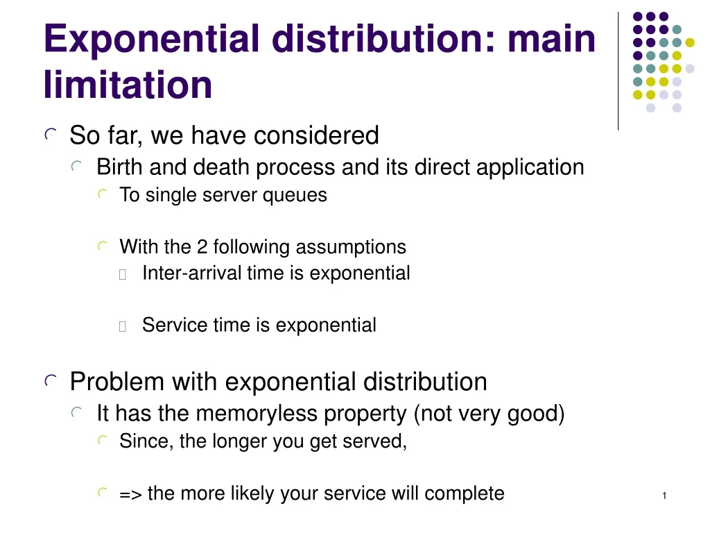
Exponential distribution: main limitation • So far, we have considered • Birth and death process and its direct application • To single server queues • With the 2 following assumptions • Inter-arrival time is exponential • Service time is exponential • Problem with exponential distribution • It has the memoryless property (not very good) • Since, the longer you get served, • => the more likely your service will complete
Exponential assumption: example • Let us consider • Queue in one of the output ports of a router • Is it ok to model this queue as an M/M/1 queue? • A lot of people do, but is it correct? • The implication of such a model • Transmission delay of a packet is exponential? • If you are doing file transfer all packets are 1500 bytes long • The latest statistics from SANs (Storage Area Networks) 1500 bytes P1 500 bytes P2 64 bytes P3
Inter-arrival time: is it exponential? • Back in the 80s • When the link speeds were very small • It was OK to consider packet arrival to be Poisson • But as speeds picked up with the advent of SONET • Because of the tremendous speed, the utilization of links • No longer regular (spaced out with exponential inter-arrival) • Instead, traffic is bursty (packets are grouped together) • You go thru an ON period with back to back packets • Followed by an off period • It is better to use Interrupted Poisson distribution
Erlang model: mixture of exponentials • Erlang • Realized • the exponential distribution • was not an adequate modeling technique • But it is important to keep it as it leads to easy mathematics • Came up with another idea • Mixture of exponentials represented by the letter E • Combine several exponentials to make up a service Break it up into r exponentials in tandem … μ rμ rμ rμ
Erlang model: main concept • The arriving customer • Takes a sequence of exponential services • Instead of a single service time • Breaking service time into r service times • Is called Er Erlang distribution with r stages • However, the r servers are equivalent to one server • Only one customer is accommodated in service at a time • Example: E2 • Why is it important? • Arbitrary pdf can be represented by the Erlang model 1/2μ 1/2μ
Coxian model: main idea • Idea • Instead of forcing the customer • to get r exponential distributions in an Er model • The customer will have the choice to get 1, 2, …, r services • Example • C2 : when customer completes the first phase • He will move on to 2nd phase with probability a • Or he will depart with probability b (where a+b=1) a b
Laplace transform • X is a continuous random variable • fX (x) is the probability density function of X • Laplace transform of X • Since,
Main property of Laplace transform • Main property • Proof: first and second moment
Moment generating functions • Laplace transform is a special case of • Moment generating function ø(t) • It is called as such because of all of the moments of X • Can be obtained by successively differentiating it • Laplace transform is obtained • t = -s
Laplace transform of an exponential distribution • Let X be a continuous random variable • That follows the exponential distribution • The Laplace transform of X is given by
Convolution of 2 discrete random variables • Let • X1 and X2 be discrete random variables • Whose probability distributions are known • P[X1 = x1] and P[X2 = x2] • Y be the sum of X1 and X2 • What is the probability distribution of Y = X1 + X2? • P[Y = y]
Convolution of 2 continuous random variables • Let X1 and X2 be 2 continuous random variables • fX1 (x1) and fX2 (x2) are known • => fX1 *(s) and fX2 *(s) are known • Let Y = X1 + X2 • What is the pdf of Y?
Application to Erlang model 1/2μ 1/2μ • X1 and X2 • are exponentially distributed and independent • with mean 1/2μ each X1 X2 Y=X1+X2
Erlang service time: first and second moment • The mean of Y? • The variance of Y? • Exercise at home • Obtain the mean and variance of E2 from • its Laplace transform
Squared coefficient of variation • The squared coefficient of variation • Gives you an insight to the dynamics of a r.v. X • Tells you how bursty your source is • C2 get larger as the traffic becomes more bursty • For voice traffic for example, C2 =18 • Poisson arrivals C2 =1 (not bursty)
Poisson arrivals vs. bursty arrivals • Why do we care • If arrival is bursty or Poisson • Bursty traffic will place havoc into your buffer • Example: router design % loss C2
Erlang, Hyper-exponential, and Coxian distributions • Mixture of exponentials • Combines a different # of exponential distributions • Erlang • Hyper-exponential • Coxian μ μ μ E4 μ Service mechanism μ1 P1 μ2 H3 P2 P3 μ3 μ μ μ μ C4
Erlang distribution: analysis 1/2μ 1/2μ • Mean service time • E[Y] = E[X1] + E[X2] =1/2μ + 1/2μ = 1/μ • Variance • Var[Y] = Var[X1] + Var[X2] = 1/4μ2 v +1/4μ2 = 1/2μ2 E2
Squared coefficient of variation: analysis constant exponential C2 • X is a constant • X = d => E[X] = d, Var[X] = 0 => C2 =0 • X is an exponential r.v. • E[X]=1/μ; Var[X] = 1/μ2 => C2 = 1 • X has an Erlang r distribution • E[X] = 1/μ, Var[X] = 1/rμ2 => C2 = 1/r • fX *(s) = [rμ/(s+rμ)]r Erlang 0 1 Hypo-exponential
Probability density function of Erlang r • Let Y have an Erlang r distribution • r = 1 • Y is an exponential random variable • r is very large • The larger the r => the closer the C2 to 0 • Er tends to infintiy => Y behaves like a constant • E5 is a good enough approximation
Generalized Erlang Er • Classical Erlang r • E[Y] = r/μ • Var[Y] = r/μ2 • Generalized Erlang r • Phases don’t have same μ … rμ rμ rμ Y … μ1 μ2 μr Y
Generalized Erlang Er: analysis • If the Laplace transform of a r.v. Y • Has this particular structure • Y can be exactly represented by • An Erlang Er • Where the service rates of the r phase • Are minus the root of the polynomials
Hyper-exponential distribution μ1 P1 • P1 + P2 + P3 +…+ Pk =1 • Pdf of X? μ2 X P2 . . Pk μk
Hyper-exponential distribution:1st and 2nd moments • Example: H2
Hyper-exponential: squared coefficient of variation • C2 = Var[X]/E[X]2 • C2 is greater than 1 • Example: H2 , C2 > 1 ?
Coxian model: main idea • Idea • Instead of forcing the customer • to get r exponential distributions in an Er model • The customer will have the choice to get 1, 2, …, r services • Example • C2 : when customer completes the first phase • He will move on to 2nd phase with probability a • Or he will depart with probability b (where a+b=1) a b
Coxian model μ2 μ3 μ4 μ1 a2 a3 a1 b1 b2 b3 μ1 b1 a1 b2 μ1 μ2 a1 a2 b3 μ1 μ2 μ3 a1 a2 a3 μ1 μ2 μ3 μ4
Coxian distribution: Laplace transform • Laplace transform of Ck • Is a fraction of 2 polynomials • The denominator of order k and the other of order < k • Implication • A Laplace transform that has this structure • Can be represented by a Coxian distribution • Where the order k = # phases, • Roots of denominator = service rate at each phase
Coxian model: conclusion • Most Laplace transforms • Are rational polynomials • => Any distribution can be represented • Exactly or approximately • By a Coxian distribution
Coxian model: dimensionality problem • A Coxian model can grow too big • And may have as such a large # of phases • To cope with such a limitation • Any Laplace transform can be approximated by a c • To obtain the unknowns (a, μ1, μ2) • Calculate the first 3 moments based on Laplace transform • And match these against those of the C2 a μ1 μ2 b=1-a