Download
1 / 26
260 likes | 284 Views
Understand warm-up periods & delete transients in simulations. Apply moving averages, choose replications wisely & achieve convergence for accurate inferences.

E N D
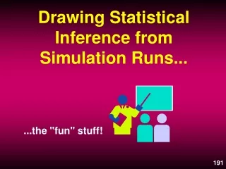
Drawing Statistical Inference from Simulation Runs... ...the "fun" stuff!
Essential Issues • Warm-up Period • Replication Determination
THE NONTERMINATING SIMULATION
Warm-up Period • Initial transient period. • When steady state is achieved • Determines deletion amount • Graphical procedure
Definitions W = Warm-up (transient) period L = Length of replication n = Number of replications m = Moving average period
Procedure • Select decision variable. (e.g. Quantity of WIP) • Make n>4 replications of duration L, where L is much larger than expected value of the transient period. • Prepare a table of observations.
Procedure • Calculate the average across each of the n periods (e.g. all day 1s, all day 2s, etc.). • Plot a moving average for m = 5, m = 10 or m = 15. • Select the warm-up period W that shows the smallest deviation from a straight line average.
Daily Number in WIP Daily Avg * Rep 1 Rep 2 Rep 3 Rep n 101 104 112 106.3 Day 1 Day 2 Day 3 Day 30 89 83 96 89.2 100 94 88 96.4 etc. * Averages are hypothetical assuming all observations are considered.
106.3 106.3 89.2 97.3 100.8 96.4 101.6 103.1 104.5 110.6 99.4 104.9 116.3 104.5 121.5 97.7 101.1 112.6 102 Daily Avg Moving Avg
125 100 75 1 30 Periods (days) Moving Average m = 5
125 100 75 Convergence 1 15 30 Periods (days) Moving Average m = 10
Clues to Success • Use n > 4 replications initially. • Keep m > L/2. • Increase replications n rather than length of run L to achieve greater smoothness. • Better to choose a warm-up period too long than too short.
THE TERMINATING SIMULATION
How Many Replications 10 ? 50 ? 100 ?
A “Quick” Method • Select your decision variable. (e.g. Average process time) • Decide how close you would like to be. “I’d like to be within +/-3 minutes of the actual process time…”
A “Quick” Method • “Estimate” the standard deviation of your decision variable... “I believe the maximum and minimum process times are 65 and 15 minutes respectively.” 65 - 15 = 50 S = 50/6 = 8.33
A “Quick” Method • Select precision level. “I want to be 95% certain of my answer” (i.e. a = .05). For 95% confidence interval, Z = 1.96.
A “Quick” Method • Solve... 2 Z * S ( ) n = 3 2 1.96 * 8.33 ( ) n = 3 n = 31
0.5 747 1066 1848 3.0 21 30 51 10.0 3 5 2 Precision Level Differences How Close 90% 95% 99% to Actual Mean (Min)
Or Use Stat::Fit
Open Stat::Fit from the Tools menu
Use the Utilities - Replications menu and fill-in the information as we did in the previous example
Number of replications