Download
1 / 69
690 likes | 704 Views
Explore advanced medical volume visualization techniques such as transfer functions, exploration of original data, and interaction tasks for detailed analysis and manipulation. Learn about synchronized displays, dynamic legends, and diverse transfer function designs for enhanced visualization experiences.

E N D
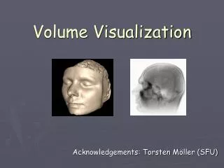
Interaction Techniques in Medical Volume Visualization Bernhard Preim
Interaction Tasks and Techniques • Interaction Tasks • Exploration of original data • Manipulation of transfer functions • Multiplanar reformatting (MPR) Bernhard Preim
Exploration of Original Data • “Browsing” through the slice data • Simple contrast and brightness control via mouse movement (windowing also called ramp transfer function) • Flexible definition of slices in a corresponding visualization • Cine mode for animation impression Bernhard Preim
Exploration of Original Data • Opening and closing of a legend in the viewer • Patient information (name, date of birth, gender, Id) • Image information (modality, voxel size, recording date) • Option: more or less detailed legend • Synchronized display of two data sets • Example: Liver CT; first data set without contrast agent, second data set with CA • Synchronization related to windowing parameters and the displayed layer • Selection of the viewing direction (coronary, sagittal, axial) Bernhard Preim
Exploration of Original Data • Example for legends, data: Univ. Hospital Leipzig Bernhard Preim
Exploration of Original Data • Change of contrast and brightness, data: Univ. Hospital Leipzig Bernhard Preim
Exploration of Original Data • Moving of a cross line in communicated views (Peter Hastreiter, Uni Erlangen) Historical model: Drawings by Dürer Bernhard Preim
Transfer Functions • Transfer functions: Mapping of data onto presentation parameters (colors, gray values, transparency) • Determine the visibility and perceptibility of structures • Parametrization of TFs is an essential interaction for the exploration of volume data. • Challenges: • Exploration of data sets with unknown structures • Exploration of data sets with different structures of similar intensity Bernhard Preim
Transfer Functions • Three volume visualizations of one CT data set with different opacity transfer functions. No exliplicit classification is applied, leading to the problems with „teeth“ Skin Bones Teeth Bernhard Preim
Transfer Functions • Requirements • Selection of predefined TFs (e.g. liver CT, lung CT) • Targeted search for suitable TFs • Correlation between adjustable parameters and characteristics of the resulting images • Definition flexibility • Fast preview Bernhard Preim
Transfer Functions • Typical transfer functions: • Windowing (ramp) • Bi-/trilevel windowing • Inverse windowing • Piecewise linear functions • Polynoms of higher degree/splines • Problem: No recognizable relation between TF characteristics and visualization Bernhard Preim
Transfer Functions • Thorax CT data set, emphasis of skeletal structures Bernhard Preim
Transfer Functions Thorax CT data set, emphasis of blood vessels Bernhard Preim
Transfer Functions • Representation and application of TFs • Discrete representation in lookup tables • Size: e.g. 4096 entries with 32 bit (8 bit each for RGB and alpha) • Hardware support for Lookup tables • Problem: hardware dependency w.r.t. size of color tables Bernhard Preim
Transfer Functions • Sophisticated concepts: • Stochastic generation of TFs that may be selected by the user (multilevel iterative search), presentation as thumbnails (He et al. [1996], König et al. [2001]) • Image-based TF design (Fang et al. [1998]) • Enhanced TF • Integration of image processing filters (e.g. edge recognition) • Local TF • Multidimensional TF (illustration of derived data, e.g. gradient fields, Levoy [1988]) Bernhard Preim
Transfer Functions • Stochastic generation of TFs: • Iterative search process (He et al. [1996]): • 1. Use of an initial TF library • 2. "Mutation" of this function through a genetic algorithm (25 generations) • 3. Direct volume rendering (back then with VolVis 100x100 pixel, 10s) • 4. Subjective result analysis by the user Bernhard Preim
Transfer Functions Source: König et al. [2001] Bernhard Preim
Transfer Functions • Image-based TF design • Idea: Definition of the transfer function, image information serve as context (Castro et al. [1998]) • Global histogram • Histogram along a layer • Histogram along a ray Bernhard Preim
Transfer Functions • Histogram along the orange ray as context for TF specification eye ball (light) muscles (dark) Image: Dirk Bartz, Univ. Leipzig Bernhard Preim
Transfer Functions • RGB Alpha and gray value Alpha TF (Courtesy of Peter Hastreiter, Univ. Erlangen) Bernhard Preim
Transfer Functions • Composition of a TF as weighted sum of component functions • Components may represent known materials, e.g. fat, bone, … • Parameters of component functions: • Sb, Sc - inner sampling points, Sa, Sd- outer sampling points Bernhard Preim
TransferFunctions • Adaptation of a trapezoid template to the local histogram of a rectangular region. Source: Castro et al. [1998] Bernhard Preim
Transfer Functions • The Transfer Function Bake-Off, Data: Sheep heart (IEEE CG&Application 5/6 2001, Pfisterer) • Comparison of different TF specification techniques • ISO rendering of the segmented raw data (sheep heart) • Trial&Error - (20 min) with VolumePro • Without data model - ISO automatically selected according to the maximum gradient magnitude • 2D TF with data model – automatic distance map, semiautom. opacity, manual color map Source: Pfisterer [2001] Bernhard Preim
Transfer Functions • Data-based Techniques • Selection of a transfer function that emphasizes edges. • Edge model: • Perfect intersection between 2 structures is "blurred" through an error function (point spread function of the data acquisition). Assumption: Blurring through an isotropic Gaussian function. → fits to CT data well • Source: Kindlman, Durkin [1998] Bernhard Preim
Transfer Functions • Data-based Techniques: edge enhancement • Edge criteria: strong gradient g, very small second derivative h (zero crossing): • -h(v) • p(v) = • g(v) • Data values along an edge, 1st and 2nd derivative Bernhard Preim
Transfer Functions • Determination of g (v) and h (v) via average determination from all first and second derivatives of all voxels with value v. • Internal representation: • Histogram volume H: • x-axis → f (v) • y-axis → f“(v) • z-axis → f´(v) • Algorithm: • 1. Determine min. and max. values • for f‘‘(v) and the maximum for f´(v). • Minimum for f´(v) is assumed to be 0. • 2. Fill H, whereas the values are scaled • such that min and max are depicted from • f´ and f´´ to 0 and 256. Bernhard Preim
Transfer Functions • Data-based Techniques: edge enhancement • What can be determined from the histogram volume? • Edge positions w.r.t. the data • What can be entered by the user? • A selection of the "peaks" that shall be depicted • Form of the depicted peaks via boundary emphasis function (bef) • Typical forms of bef() Bernhard Preim
Transfer Functions • Data-basedTechniques: edgeenhancement • Applied 2D opacityfunction • and volumerendering of the • Visible Womandataset • (TF automaticallydetermined). • The smallimageindicates the 2D • Histogram (intensityvalues vs. • gradientmagnitude) • Brightness indicatesfrequency of the • combination. • Source: Kindlmann, Durkin (1998) Bernhard Preim
Transfer Functions • Data-based Techniques: edge enhancement • Comparison of edge-enhancing direct volume rendering and iso-surface rendering Illustration of a spiny dendrite based on microscopy data • Source: Kindlmann and Durkin 1998 Bernhard Preim
Transfer Functions • Data-based Techniques: edge enhancement • Preconditions for successful application: • Existence of clear object boundaries • Homogenous data • Only little noise, no "outliers" • Medicine: CT data (if CA is applied, it must be equally distributed) Bernhard Preim
Transfer Functions • Data-basedTechniques • Useof a oncespecified TF asreference • Goal: "Re-use" of an empiricallyspecified TF • Application: targetedillustrationof a structure in a modality (e.g. aneurysms in MR) • Procedure: • Selection of a referencedatasetDrefand a TFTref(v) • UseofthenormalizedhistogramsofthedatasetsH(Dref) andH(Dstudy) • Non-linear transformationt of the intensity values of Dstudy, such thatH (Dstudy) ~ H (t(Dref)) • Hence, Tstudy (v) = Tref (v) Bernhard Preim
Transfer Functions • Data-based Techniques: reference TF • Determination of the similarity of the histograms • 1. Idea: minimization of the histogram distances • 2. Better idea: use of the p-function by Kindlmann (considers also f‘(v) and f‘‘(v)) • In case of comparable data sets the p-values are similar to the histograms • Literature: Rezk-Salama et al., VMV [2000] Bernhard Preim
Transfer Functions • Data-based Techniques: Reference TF • Visualization of blood vessels in the brain with CT angiography, left: no adaptation, middle: illustration of the first idea (histogram transformation), right: adaptation of the p-function Source: Rezk-Salama et al. [2000] Bernhard Preim
Transfer Functions • Multidimensional TFs • 1D TF: Map data onto opacity/colors • Multidimensional TFs: Use additionally derived information, e.g. strength of the gradient or the second derivative • Typical example: Adaptation of the opacity to the strength of the gradient, emphasis of data intersections • Advantage: Additional degrees of freedom to generate high-quality images • Disadvantage: High interaction costs Bernhard Preim
Transfer Functions • Multidimensional TFs • Consideration of the 2nd derivative (1st derivative of a scalar field → vector, 2nd derivative → matrix) • Hessian Matrix: • Criterion (scalar value) for the 2nd derivative: largest eigenvalue of the Hessian Matrix and strength of the 2nd derivative, respectively in direction to the gradient (instead of the Hessian Matrix) Bernhard Preim
Transfer Functions • Multidimensional TFs • Gradient calculation usually via central differences • Mapping of the gradient size to the opacity (gradient magnitude weighted transparency) Bernhard Preim
Transfer Functions • Multidimensional TFs • Volume visualization with a gradient-dependent TF for opacity, according to Levoy [1988]) (Visible Human CT data set) Bernhard Preim
2D Transfer Functions • Starting point for a simple specification: gradient intensity histograms. Filtering is important. Goal: accentuation of intersections. Source: Stölzl [2004] Bernhard Preim
2D Transfer Functions Dense tissue and bone parts with additional gradient emphasis (green marking) Image courtesy: Hoen-Oh Shin and Benjamin King, MH Hannover [2004] Bernhard Preim
2D Transfer Functions More dense soft tissue (yellow marking) Image courtesy: Hoen-Oh Shin and Benjamin King, MH Hannover [2004] Bernhard Preim
2D Transfer Functions Regions with high gradients are visualized (red marking) Image courtesy: Hoen-Oh Shin and Benjamin King, MH Hannover [2004] Bernhard Preim
2D Transfer Functions • Edge detector as input to define arcs Source: Stölzl [2004] Bernhard Preim
2D Transfer Functions • Local TFs • Motivation: Often, global TFs enable no sufficient differentiation • Another kind of 2D TFs with the 2nd dimension being the object id • Example: Division of a lookup table into 4 segments for 4 different illustrations Caution: Interpolation beyond segment borders is not allowed! Source: Rezk-Salama [2002] Bernhard Preim
2D Transfer Functions • Blood vessels in the lung lobes are displayed with separate local TFs. Bernhard Preim
2D Transfer Functions • Template-based specification of 2D TFs • 1D templates: • 2D templates: Source: Castro et al. [1998] Source: Tappenbeck [2006] Bernhard Preim
2D Transfer Functions • Template-based specification of 2D TFs: • Simplification of the interaction is even more important than in the 1D case • Discretization in a Lookup table • Sufficient size required, at least 256x256 • Applicable to arbitrary 2D domains (intensity: gradient strength, intensity: distance to a target structure, …) Bernhard Preim
2D Transfer Functions • Representation of 2D TFs in a rectilinear grid as basis for discretization in an LUT Source: Tappenbeck [2006] Bernhard Preim
2D Transfer Functions • Distance-dependent TFs: • Additional entries: • Segmented target structure (tagged volume) • Distance transformation w.r.t. the target • Use of an editor for 2D TF • Sample applications: • Fade-in of safety margins around tumors • Opacity control in case of large organs Bernhard Preim
2D Transfer Functions • Target structure: lung surface • Selection of interesting structures by intensity and distances Source: Tappenbeck [2006] Bernhard Preim
2D Transfer Functions • Resulting Volume Visualization (quite useless example; but appropriate illustration of the concept). Distance to the lung is used to assign different colors and opacity values. Source: Tappenbeck [2006] Bernhard Preim