Introduction to Volume Visualization
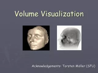
Introduction to Volume Visualization . Mengxia Zhu Fall 2007. Volume Visualization . Volume visualization is used to create images from volumetric data defined on multiple dimensional grids

Introduction to Volume Visualization
E N D
Presentation Transcript
Introduction to Volume Visualization Mengxia Zhu Fall 2007
Volume Visualization • Volume visualization is used to create images from volumetric data defined on multiple dimensional grids • volumetric data is typically a set of samples f(x,y,z,d) with d representing the data property at a location determined by (x,y,z). • Timing varying volumetric data f(x, y, z, t, d)
Data Type • d can take the form of scalar, vector, or even tensor. • Scalar, Single valued at each location in a dataset. Examples are temperature, pressure, density, and elevation etc. Simplest and most common form. i.e. f of type real, integer • Vector, data with magnitude and direction. In 3D, it is represented as a triplet of values ( u,v,w). Examples include flow velocity, particle trajectory, wind motion, and gradient function. • Tensor, complex mathematical generalizations of vectors and matrices. A tensor of rank 0 is a scalar. Rank 1 is vector, rank 2 is 3x3 matrix. • E.g. stress and strain in FEM modeling, which represent the stress and strain at a point in an object under load
Data Elements • Volumetric data is usually defined on a cartesian grid • two alternative methods defining data elements. • Voxels: sample values are called voxel • Cells: a cuboidal region with voxels at 8 grid corners.
Regular and Irregular Structure • A dataset consists of an organizing structure and associated attribute data • Characterized according to whether its structure is regular or irregular. • If there is a single mathematical relationship within the composing points and cells, a dataset is regular. • Regular data can be implicitly represented efficiently. • Irregular data must be explicitly represented since there is no inherent pattern that can be compactly described. Unstructured data tends to be more general, but requires greater memory and computational resources.
Grid and Lattice • Cartesian grids: all elements are identical axis-aligned cubes • Regular grid: identical rectangular elements aligned along the axes of the dataset. • Rectilinear Grids: aligned along the axes of the dataset. However arbitrary spacing and the data elements themselves are no longer identical. • curvilinearGrids: Elements are no longer axis aligned, and again the elements can be non-identical.
Grid Types Structured Grids: uniform regular rectilinear curvilinear Unstructured Grids: regular irregular hybrid curved
Examples Regular grid Rectilinear grid
Methods • The fundamental algorithms are of two types: • direct volume rendering (DVR) algorithms • surface-fitting (SF) algorithms. • DVR methods map elements directly into screen space without using intermediate geometric primitives as an intermediate representation. • SF methods are also called feature-extraction or iso-surfacing and fit planar polygons or surface patches to constant-value contour surfaces.
www.cs.sunysb.edu/.../ WeiWeb/research.htm www.mpa-garching.mpg.de/ gadget/hydrosims/ www-vis.lbl.gov/.../ ChomboVis99/sharedvrend.html
DVR versus SF • Volume rendering is a process of creating a 2D image directly from 3D volumetric data • Mapping the entire 3D data into a 2D image • SF is a process of creating an image of a surface contained within the volume data using geometric primitives • Marching Cubes algorithm (triangles as primitives) • Dividing Cubes algorithm (3D points as primitives) • DVR conveys more information than surface rendering images at the cost of increased algorithm complexity and rendering times • Volume rendering to display amorphous phenomena such as clouds, fog
Direct Volume Rendering Techniques • Object-order technique • Uses a forward mapping scheme where the volume data is mapped into the image plane • Image-order technique • Uses a backward mapping scheme where rays are cast from each pixel in the image plane through the volume data to determine the pixel value • Hybrid technique • Combines the two approaches
Data Classification • Threshold value (Iso-value) for an SF method or the color and opacity values (transfer function) for a DVR method. • The DVR color table is used to map data values to meaningful colors. The opacity table is used to expose the part of the volume most interesting to the user and to make transparent the uninteresting parts.
Common Steps in SF • Data acquisition either via empirical measurement or computer simulation. • Put the data into a format that can be easily manipulated. This may entail scaling the data for a better value distribution, enhancing contrast, filtering out noise, and removing out-of-range data. • The data is mapped onto geometric or display primitives. • The primitives are stored, manipulated, and displayed.
Interpolation • Interpolation assumes that the value of the data element varies across the element. some combination of the surrounding grid points. • For example, with trilinearinterpolation the value at a arbitrary point in the data element is calculated from the surrounding eight grid points.
Trilinear Interpolation Trilinear interpolation is the process of taking a three-dimensional set of numbers and interpolating the values linearly, finding a point using a weighted average of eight values.
Shading • To create a realistic image, shading with light define how much light each data point received. • The gradient is used to approximate the surface normal to an imaginary surface touching the point. • Central difference method: