Download
1 / 52
520 likes | 541 Views
Explore benchmarking of gate sizing heuristics using eyechart topologies to optimize power, speed, area, and leakage power under timing constraints. Study suboptimality, existing heuristics, and solve combinational circuit challenges.

E N D
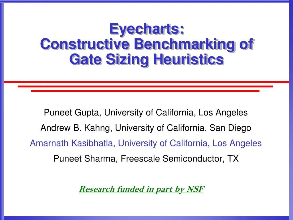
Eyecharts: Constructive Benchmarking of Gate Sizing Heuristics Puneet Gupta, University of California, Los Angeles Andrew B. Kahng, University of California, San Diego Amarnath Kasibhatla, University of California, Los Angeles Puneet Sharma, Freescale Semiconductor, TX Research funded in part by NSF
Outline 2 • Motivation • Solving Eyechart Topologies • Experiments for Suboptimality Study • Results
Why is Sizing Important? 3 • Sizing • Effective way of optimizing for power, speed and area • Tunable parameters • Gate-width • Threshold voltage • Gate-length • Supply voltage etc. • Sizing problem seen at all stages of RTL to GDS flow • Power recovery crucial during post-layout phase
Why Study Suboptimality? 4 • Literally hundreds of gate sizing methods exist • Common heuristics/algorithms: • Linear Programming, Lagrangian Relaxation, Convex Optimization, Dynamic Programming, Geometric Programming, Sensitivity based gradient-descent, Simulated Annealing etc. • Which heuristic is better? • No systematic way to compare, so far • How suboptimal are these heuristics? • Does a heuristic’s performance depend on • Circuit topology? • Characteristics of the cell library? • No prior work focuses on these aspects
Sizing Problem Formulation 5 • Sizing problem could be discrete or continuous • Discrete sizing problem is NP-hard • Common designs are standard cell-based and discrete • We focus only on discrete sizing problem • Problem: Leakage power minimization under timing constraints • Circuits are purely combinational • Gate sizing alone is tested and not logic optimization capability
Our Contributions 6 • We generate artificial combinational circuits called eyecharts • Gate’s delay depends only on • Gate size • Total load capacitance • Eyecharts can be solved optimally using Dynamic Programming (DP) • A variety of eyecharts are generated by varying • Circuit topology • Power-Size, delay-size characteristics of library • Suboptimalities of existing heuristics studied under these variations • Leakage optimization details are presented • Extensions to dynamic power optimization are easy
Outline 7 • Motivation • Solving Eyechart Topologies • Experiments for Suboptimality Study • Results
What are Eyecharts? 8 • Chain, Mesh and Star proposed • Each can be solved optimally for the assumed delay model • Stage of a gate is its logic level from the PI • Levelized nature of eyecharts enables optimal sizing by DP Chain MESH STAR
What are Eyecharts? 9 • Chain, Mesh and Star proposed • Each can be solved optimally for the assumed delay model • Stage of a gate is its logic level from the PI • Levelized nature of eyecharts enables optimal sizing by DP Chain Stage3 Stage4 Stage2 Stage5 Stage1 PO PI MESH STAR
Solving a Chain Optimally 10 Input Leakage Delay cap power Load Load = 3 = 6 Size 1 3 5 3 4 Size 2 6 10 1 2
Solving a Chain Optimally 11 Stage 3 Stage 2 Input Leakage Delay cap power Load Load 3 6 Size 1 3 5 3 4 Size 2 6 10 1 2 Stage 1 Dmax = 8 6 INV3 INV1 INV2
Solving a Chain Optimally 12 Stage 3 Stage 2 Input Leakage Delay cap power Load Load 3 6 Size 1 3 5 3 4 Size 2 6 10 1 2 Stage 1 Dmax = 8 ? 6 INV3 INV1 INV2
Solving a Chain Optimally 13 Stage 3 Stage 2 Input Leakage Delay cap power Load Load 3 6 Size 1 3 5 3 4 Size 2 6 10 1 2 Stage 1 Dmax = 8 ? 6 INV3 INV1 INV2 Stage 1 Budget Power Size 1 ? ? 2 ? ? 3 ? ? 4 ? ? 5 ? ? 6 ? ? 7 ? ? 8 ? ?
Solving a Chain Optimally 14 Stage 3 Stage 2 Input Leakage Delay cap power Load Load 3 6 Size 1 3 5 3 4 Size 2 6 10 1 2 Stage 1 Dmax = 8 ? 6 INV3 INV1 INV2 Stage 1 Budget Power Size 1 ? ? 2 ? ? 3 ? ? 4 ? ? 5 ? ? 6 ? ? 7 ? ? 8 ? ? Load = 3
Solving a Chain Optimally 15 Stage 3 Stage 2 Input Leakage Delay cap power Load Load 3 6 Size 1 3 5 3 4 Size 2 6 10 1 2 Stage 1 Dmax = 8 ? 6 INV3 INV1 INV2 Stage 1 Budget Power Size 2 ? ? 3 ? ? 4 ? ? 5 ? ? 6 ? ? 7 ? ? 8 ? ? Load = 6
Solving a Chain Optimally 16 Stage 3 Stage 2 Input Leakage Delay cap power Load Load 3 6 Size 1 3 5 3 4 Size 2 6 10 1 2 Stage 1 Dmax = 8 ? 6 INV3 INV1 INV2 Stage 1 Budget Power Size 1 ? ? 2 ? ? 3 ? ? 4 ? ? 5 ? ? 6 ? ? 7 ? ? 8 ? ? Load = 3 2 ? ? 3 ? ? 4 ? ? 5 ? ? 6 ? ? 7 ? ? 8 ? ? Load = 6
Solving a Chain Optimally 17 Stage 3 Stage 2 Input Leakage Delay cap power Load Load 3 6 Size 1 3 5 3 4 Size 2 6 10 1 2 Stage 1 Dmax = 8 ? 6 INV3 INV1 INV2 Stage 1 Budget Power Size 1 ? ? 2 ? ? 3 ? ? 4 ? ? 5 ? ? 6 ? ? 7 ? ? 8 ? ? Load = 3 2 ? ? 3 ? ? 4 ? ? 5 ? ? 6 ? ? 7 ? ? 8 ? ? Load = 6
Solving a Chain Optimally 18 Stage 3 Stage 2 Input Leakage Delay cap power Load Load 3 6 Size 1 3 5 3 4 Size 2 6 10 1 2 Stage 1 Dmax = 8 ? 6 INV3 INV1 INV2 Stage 1 Budget Power Size 1 ? ? 2 ? ? 3 ? ? 4 ? ? 5 ? ? 6 ? ? 7 ? ? 8 ? ? Load = 3 2 ? ? 3 ? ? 4 ? ? 5 ? ? 6 ? ? 7 ? ? 8 ? ? Load = 6
Solving a Chain Optimally 19 Stage 3 Stage 2 Input Leakage Delay cap power Load Load 3 6 Size 1 3 5 3 4 Size 2 6 10 1 2 Stage 1 Dmax = 8 6 INV3 INV1 INV2 Stage 1 Budget Power Size 1 ? ? 2 ? ? 3 5 1 4 ? ? 5 ? ? 6 ? ? 7 ? ? 8 ? ? Load = 3 2 ? ? 3 ? ? 4 ? ? 5 ? ? 6 ? ? 7 ? ? 8 ? ? Load = 6
Solving a Chain Optimally 20 Stage 3 Stage 2 Input Leakage Delay cap power Load Load 3 6 Size 1 3 5 3 4 Size 2 6 10 1 2 Stage 1 Dmax = 8 6 INV3 INV1 INV2 Stage 1 Budget Power Size 1 10 2 2 10 2 3 5 1 4 5 1 5 5 1 6 5 1 7 5 1 8 5 1 Load = 3 2 10 2 3 10 2 4 5 1 5 5 1 6 5 1 7 5 1 8 5 1 Load = 6
Solving a Chain Optimally 21 Stage 3 Stage 2 Input Leakage Delay cap power Load Load 3 6 Size 1 3 5 3 4 Size 2 6 10 1 2 Stage 1 Dmax = 8 6 INV3 INV1 INV2 Stage 1 Stage 2 Budget Power Size Budget Power Size 3 20 2 4 15 1 5 15 2 6 10 1 7 10 1 8 10 1 1 10 2 2 10 2 3 5 1 4 5 1 5 5 1 6 5 1 7 5 1 8 5 1 Load = 3 Load = 3 2 10 2 3 10 2 4 5 1 5 5 1 6 5 1 7 5 1 8 5 1 4 20 2 5 15 1 6 15 2 7 10 1 8 10 1 Load = 6 Load = 6
Solving a Chain Optimally 22 Stage 3 Stage 2 Input Leakage Delay cap power Load Load 3 6 Size 1 3 5 3 4 Size 2 6 10 1 2 Stage 1 Dmax = 8 6 INV3 INV1 INV2 Stage 1 Stage 2 Budget Power Size Budget Power Size 3 20 2 4 15 1 5 15 2 6 10 1 7 10 1 8 10 1 1 10 2 2 10 2 3 5 1 4 5 1 5 5 1 6 5 1 7 5 1 8 5 1 Load = 3 Load = 3 2 10 2 3 10 2 4 5 1 5 5 1 6 5 1 7 5 1 8 5 1 4 20 2 5 15 1 6 15 2 7 10 1 8 10 1 Load = 6 Load = 6
Solving a Chain Optimally 23 Stage 3 Stage 2 Input Leakage Delay cap power Load Load 3 6 Size 1 3 5 3 4 Size 2 6 10 1 2 Stage 1 Dmax = 8 6 INV3 INV1 INV2 Stage 1 Stage 2 Budget Power Size Budget Power Size 3 20 2 4 15 1 5 15 2 6 10 1 7 10 1 8 10 1 1 10 2 2 10 2 3 5 1 4 5 1 5 5 1 6 5 1 7 5 1 8 5 1 Load = 3 Load = 3 INV2 Excess Total delay budget power size 1 3 3 10 2 10 2 3 10 2 4 5 1 5 5 1 6 5 1 7 5 1 8 5 1 4 20 2 5 15 1 6 15 2 7 10 1 8 10 1 Load = 6 Load = 6
Solving a Chain Optimally 24 Stage 3 Stage 2 Input Leakage Delay cap power Load Load 3 6 Size 1 3 5 3 4 Size 2 6 10 1 2 Stage 1 Dmax = 8 6 INV3 INV1 INV2 Stage 1 Stage 2 Budget Power Size Budget Power Size 3 20 2 4 15 1 5 15 2 6 10 1 7 10 1 8 10 1 1 10 2 2 10 2 3 5 1 4 5 1 5 5 1 6 5 1 7 5 1 8 5 1 Load = 3 Load = 3 INV2 Excess Total delay budget power size 1 3 3 10 size 2 1 5 15 2 10 2 3 10 2 4 5 1 5 5 1 6 5 1 7 5 1 8 5 1 4 20 2 5 15 1 6 15 2 7 10 1 8 10 1 Load = 6 Load = 6
Solving a Chain Optimally 25 Stage 3 Stage 2 Input Leakage Delay cap power Load Load 3 6 Size 1 3 5 3 4 Size 2 6 10 1 2 Stage 1 Dmax = 8 6 INV3 INV1 INV2 Stage 3 Stage 1 Stage 2 Budget Power Size Budget Power Size Budget Power Size Load = 6 3 20 2 4 15 1 5 15 2 6 10 1 7 10 1 8 10 1 1 10 2 2 10 2 3 5 1 4 5 1 5 5 1 6 5 1 7 5 1 8 5 1 8 20 1 Load = 3 Load = 3 2 10 2 3 10 2 4 5 1 5 5 1 6 5 1 7 5 1 8 5 1 4 20 2 5 15 1 6 15 2 7 10 1 8 10 1 Load = 6 Load = 6
Solving a Chain Optimally 26 Stage 3 Stage 2 Input Leakage Delay cap power Load Load 3 6 Size 1 3 5 3 4 Size 2 6 10 1 2 Stage 1 Dmax = 8 6 INV3 INV1 INV2 Stage 3 Stage 1 Stage 2 Budget Power Size Budget Power Size Budget Power Size Load = 6 3 20 2 4 15 1 5 15 2 6 10 1 7 10 1 8 10 1 1 10 2 2 10 2 3 5 1 4 5 1 5 5 1 6 5 1 7 5 1 8 5 1 8 20 1 Load = 3 Load = 3 INV3 Excess Total delay budget power size 1 4 4 20 size 2 2 6 25 2 10 2 3 10 2 4 5 1 5 5 1 6 5 1 7 5 1 8 5 1 4 20 2 5 15 1 6 15 2 7 10 1 8 10 1 Load = 6 Load = 6
Solving a Chain Optimally 27 Stage 3 Stage 2 Input Leakage Delay cap power Load Load 3 6 Size 1 3 5 3 4 Size 2 6 10 1 2 Stage 1 Dmax = 8 6 INV3 INV1 INV2 Stage 3 Stage 1 Stage 2 Budget Power Size Budget Power Size Budget Power Size Load = 6 3 20 2 4 15 1 5 15 2 6 10 1 7 10 1 8 10 1 1 10 2 2 10 2 3 5 1 4 5 1 5 5 1 6 5 1 7 5 1 8 5 1 8 20 1 Load = 3 Load = 3 INV3 Excess Total delay budget power size 1 4 4 20 size 2 2 6 25 2 10 2 3 10 2 4 5 1 5 5 1 6 5 1 7 5 1 8 5 1 4 20 2 5 15 1 6 15 2 7 10 1 8 10 1 Load = 6 Load = 6
Solving a Chain Optimally 28 Stage 3 Stage 2 Input Leakage Delay cap power Load Load 3 6 Size 1 3 5 3 4 Size 2 6 10 1 2 Stage 1 Dmax = 8 6 INV3 INV1 INV2 Stage 3 Stage 1 Stage 2 Budget Power Size Budget Power Size Budget Power Size Load = 6 3 20 2 4 15 1 5 15 2 6 10 1 7 10 1 8 10 1 1 10 2 2 10 2 3 5 1 4 5 1 5 5 1 6 5 1 7 5 1 8 5 1 8 20 1 Load = 3 Load = 3 INV3 Excess Total delay budget power size 1 4 4 20 size 2 2 6 25 2 10 2 3 10 2 4 5 1 5 5 1 6 5 1 7 5 1 8 5 1 4 20 2 5 15 1 6 15 2 7 10 1 8 10 1 Load = 6 Load = 6
Solving a Chain Optimally 29 Stage 3 Stage 2 Input Leakage Delay cap power Load Load 3 6 Size 1 3 5 3 4 Size 2 6 10 1 2 Stage 1 Dmax = 8 6 INV3 INV1 INV2 Stage 3 Stage 1 Stage 2 Budget Power Size Budget Power Size Budget Power Size Load = 6 3 20 2 4 15 1 5 15 2 6 10 1 7 10 1 8 10 1 1 10 2 2 10 2 3 5 1 4 5 1 5 5 1 6 5 1 7 5 1 8 5 1 8 20 1 Load = 3 Load = 3 2 10 2 3 10 2 4 5 1 5 5 1 6 5 1 7 5 1 8 5 1 4 20 2 5 15 1 6 15 2 7 10 1 8 10 1 Load = 6 Load = 6
Solving a Chain Optimally 30 Stage 3 Stage 2 Input Leakage Delay cap power Load Load 3 6 Size 1 3 5 3 4 Size 2 6 10 1 2 Stage 1 Dmax = 8 6 INV3 INV1 INV2 Stage 3 Stage 1 Stage 2 Budget Power Size Budget Power Size Budget Power Size Load = 6 3 20 2 4 15 1 5 15 2 6 10 1 7 10 1 8 10 1 1 10 2 2 10 2 3 5 1 4 5 1 5 5 1 6 5 1 7 5 1 8 5 1 8 20 1 Load = 3 Load = 3 6fF OPTIMIZED CHAIN 2 10 2 3 10 2 4 5 1 5 5 1 6 5 1 7 5 1 8 5 1 4 20 2 5 15 1 6 15 2 7 10 1 8 10 1 Load = 6 Load = 6
Solving Mesh Optimally 31 • Stage with multiple gates represented with composite cell Stage3 Stage2 Stage4 A1 Stage1 Stage5 B1 A2 B2 A1 B1 A1 B2 A2 A1 B2 C2 C3 C4 • Mesh to chain conversion
Solving Mesh Optimally 32 • Stage with multiple gates represented with composite cell • Delay, power numbers for all size combinations for all output load combinations Delay, power table of B1 Stage3 Input Power Delay cap Load Load =12 = 24 Size 1 6 10 6 8 Size 2 12 20 2 4 Stage2 Stage4 A1 Stage1 Stage5 B1 A2 B2 A1 B1 A1 B2 LOAD = 24 LOAD = 12 A2 Size Power Delay (B1,B2) (1,1) 30 12 (1,2) 50 6 (2,1) 40 12 (2,2) 60 4 Size Power Delay (B1,B2) (1,1) 30 16 (1,2) 50 8 (2,1) 40 16 (2,2) 60 8 STAGE 4 A1 B2 C2 C3 C4 • Mesh to chain conversion
Solving Star Optimally 33 • Star solved by converting it to chain • Composite cells formed for stages with multiple gates A1 A2 B A1 A2 B C1 C3 A1 A2 C1 & C3, Composite cells for Stages 1 & 3 Stage2 Stage 3 Stage 1
Hybrid Eyecharts 34 • Chain, mesh, star daisy-chained for arbitrarily large hybrid eyecharts • Mesh/chain arbitrarily inserted along each PI/PO chain • Hybrid eyechart solved optimally by ultimately reducing it to a chain Sample hybrid eyechart A A A A B B PI1 PO1 A A B A A A A B A B B C A B A B A Chain 3 Chain 1 A A A A B A B PI2 PO2 A B A B A A A B B A B A B Chain 2 Chain 4 A A C Chain 1 and Chain 2 Chain 3 and Chain 4
Arbitrary Extensions to Eyecharts 35 • Arbitrary extensions potentially add more realism to eyecharts • Such topologies solved using partial enumeration • No levelization restriction • One example is multi-output mesh PO PI MESH
Arbitrary Extensions to Eyecharts 36 • Arbitrary extensions potentially add more realism to eyecharts • Such topologies solved using partial enumeration • No levelization restriction • One example is multi-output mesh PO PI MESH PO 1 PO 2 PI PO 3 MULTI-OUTPUT MESH
Arbitrary Extensions to Eyecharts 37 • Arbitrary extensions potentially add more realism to eyecharts • Such topologies solved using partial enumeration • No levelization restriction • One example is multi-output mesh PO PI MESH PO 1 PO 2 PI PO 3 MULTI-OUTPUT MESH
Outline 38 • Motivation • Solving Eyechart Topologies • Experiments for Suboptimality Study • Results
Experimental Setup 39 • Heuristics compared • Comm1, Comm2: Two different commercial gate-sizing/leakage-optimization tools • GS: Sensitivity-based sizing tool with sensitivity metric = • LP: Linear programming tool [Nguyen et.al, ISLPED ’03] • SBS: Sensitivity-based sizing tool with sensitivity metric = [Gupta et.al, IEEE Tran. on CAD ’06] • Explored power, delay tradeoffs with size • LP-LD: Linear increase in power, linear increase in delay • LP-NLD: Linear increase in power, nonlinear increase in delay • EP-LD: Exponential increase in power, linear increase in delay • EP-NLD: Exponential increase in power, nonlinear increase in delay • Experiments to explore dependence of suboptimality on • Circuit size, circuit topology • Delay-Size, power-size tradeoff • Granularity of the cell library
Library Characteristics 40 • The sizing choices for EP-LD and EP-NLD models are Vt variants and gate-length variants • Capacitance does not vary across Vt variants • Capacitance increase with gate-length for gate-length variants • Delay values are fitted to a 65 nm industrial library • Suboptimalities are calculated as Library Model RMS fitting Optimization Default # error (delay) context sizes/variants LP-LD 8.43% Gate Sizing 8 LP-NLD 0.3% Gate Sizing 8 EP-LD 8.43% Vt, gate-length 3,3 EP-NLD 0.3% Vt, gate-length 3,3
Outline 41 • Motivation • Solving Eyechart Topologies • Experiments for Suboptimality Study • Results
Circuit Topology Impact 42 Mesh-only Star-only Chain-only Suboptimality % • Mesh is the toughest topology
Circuit Size Impact 43 • Suboptimality relatively constant with circuit size • 10K-gate benchmarks for the rest of the experiments • LP runtime does not scale well #Gates Comm1 RT Comm2 RT LP RT GS RT % % % % 1796 21.31 14 15.81 16 15.7 56 23.1 24 10026 21.29 261 16.73 365 15.5 450 23.5 309 25993 20.98 540 15.75 539 15.4 1617 23.2 512 51015 21.3 721 16.21 722 15.1 2458 23.5 921
Circuit Size Impact 44 • Suboptimality relatively constant with circuit size • 10K-gate benchmarks for the rest of the experiments • LP runtime does not scale well #Gates Comm1 RT Comm2 RT LP RT GS RT % % % % 1796 21.31 14 15.81 16 15.7 56 23.1 24 10026 21.29 261 16.73 365 15.5 450 23.5 309 25993 20.98 540 15.75 539 15.4 1617 23.2 512 51015 21.3 721 16.21 722 15.1 2458 23.5 921
Impact of Timing Constraints 45 • LP-LD delay model: Linear increase in delay with size • Suboptmalities are close to zero for very tight or very relaxed constraints
Impact of Nonlinearity in Delay 46 • LP-NLD delay model: Nonlinear increase in delay with size • Gap between sensitivity-based methods and LP tool becomes narrow
Impact of Power Tradeoff 47 • EP-NLD delay model: Exponential increase in power • LP suffers significantly due to snapping error
Gate-length Biasing Scenario 48 • Tools in general slightly worse compared to Vt assignment • Capacitance varies across gate-length variants
Effect of Granularity 49 • Higher granularity has much larger benefits for exponential compared to linear power tradeoff LP-NLD EP-NLD
Extensions to Slew Dependent Delay • Delay of a gate depends on input slew • Output slew of a gate depends on • Gate size • Output load capacitance • Slew propagation is not considered • Optimal solution not guaranteed due to the need to maintain slew consistency • Experiments show suboptimality is still significant (5% to 35%)