Download
1 / 15
200 likes | 511 Views
L i near discriminant analysis (LDA). Katarina Berta katarinaberta@gmail.com bk113255m@student.etf.rs. Introduction. Fisher ’s Linear Discriminant Analysis Paper from 1936. ( link ) Statistical technique for classification LDA = two classes MDA = multiple classes

E N D
Linear discriminant analysis(LDA) Katarina Berta katarinaberta@gmail.com bk113255m@student.etf.rs
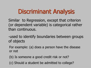
Introduction • Fisher’s LinearDiscriminant Analysis • Paper from 1936. (link) • Statistical technique for classification • LDA = two classes • MDA = multiple classes • Used in statistics, pattern recognition, machine learning
Purpose • Discriminant Analysis classifies objects in two or more groups according to linear combination of features • Feature selection • Which set of features can best determine group membership of the object? • dimension reduction • Classification • What is the classification rule or model to best separate those groups?
Method (1) Good separation Bad separation
Method (2) • Maximize the between-class scatter • Difference of mean values (m1-m2) • Minimize the within-class scatter • Covariance Min Min Max
Formula Idea: x–object i, j – classes, groups Bayes' theorem Derivation: probability density functions -normaly distributet- QDA - quadratic discriminant analysis Mean value Covarinace Σy = 0 = Σy = 1 = Σequal covarinaces FLD
Example Factory for high quality chip rings Training set
Normalization of data Training data Mean corrected data Avrage
Covarinace Covarinace for class i Covarinace class 1 – C1 Covarinace class 2 – C2 Oneentry of covarinace matrix -C covarinace matrix - C Inverse covarinace matrix C - S
Mean values N – number of objects P(i) – prior probability m1 – mean value matrix of class 1 (m(x1), m(x2)) m2 – mean value matrix of class 2 (m(x1), m(x2)) m1-m2 W= S*(m1-m2) S- inverse covariance = * W0= ln[P(1)\P(2)]-1\2*(m1+m2) = -17,7856
Resault score= X*W + W0 = + * W0
Prediction • New chip: curvature = 2.81, diameter = 5.46 • Predicition: will not pass • Prediction correct! W= S*(m1-m2) score= X*W + W0 score= -0,036 If (score>0) then class1 else class2 score= -0,036 => class2
Pros & Cons • Cons • Old algorithm • Newer algorithms - much better predicition • Pros • Simple • Fast and portable • Still beats some algorithms (logistic regression) when its assumptions are met • Good to use when begining a project
Conclusion • FisherFace one of the best algorithms for face recognition • Often used for dimension reduction • Basis for newer algorithms • Good for beginig of data mining projects • Thoug old, still worth trying
Thank you for your attention! Questions?