Arctic System Reanalysis: Land Surface Parameter Assimilation and Model Updates
390 likes | 574 Views
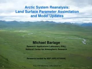
Arctic System Reanalysis: Land Surface Parameter Assimilation and Model Updates. Michael Barlage Research Applications Laboratory (RAL) National Center for Atmospheric Research Research funded by NSF ( ARC- 0733058 ). Polar WRF Workshop – 3 November 2011.

Arctic System Reanalysis: Land Surface Parameter Assimilation and Model Updates
E N D
Presentation Transcript
Arctic System Reanalysis:Land Surface Parameter Assimilation and Model Updates Michael Barlage Research Applications Laboratory (RAL) National Center for Atmospheric Research Research funded by NSF (ARC-0733058) Polar WRF Workshop – 3 November2011
Enhancements/Additions to WRF within ASR • Land surface state spin-up: more consistent initialization, less time for soil states in lower boundary to equilibrate • Changes to model structure: add more and deeper soil layers, zero-flux lower boundary condition • Land surface parameter and state assimilation: snow cover and snow depth, albedo, and green vegetation fraction inserted into model daily/weekly
Land Surface State Spin-up • Why is this necessary? • Land surface models have their own climatology • Soil layers depths between models may be inconsistent • Vegetation types, soil types, terrain, etc. are likely different between models • Land surface equilibrium can take over one year for 4-layer soil with 2 meter depth • Five year spin-up for 10-layer with 8.5 meter depth
Land Surface State Spin-up • Use High Resolution Land Data Assimilation System (HRLDAS) with atmospheric forcing from reanalysis • HRLDAS: uses WRF model grid and static fields (land cover, soil type, parameter tables) to run an offline version of the Noah LSM • Use 6-hourly reanalysis output (precipitation, wind, temperature, pressure, humidity, shortwave and longwave radiation) from ERA-40 (1980 – 1999) and JRA-25 (2000 – 2009) • Spatially interpolate forcing fields to WRF grid and adjust temperature for terrain height differences between reanalysis and WRF • Use hourly timestep by linearly interpolating all but solar radiation; the total 24hr radiation is fit to a daily zenith angle curve • Advantages are that initial fields (especially soil ice/moisture/temperature): • are already on the WRF grid • are consistent with terrain, land cover and soil types/levels • are consistent with WRF land model
Land Surface State Spin-up • August 2008 volumetric soil moisture in top and bottom layer for ERA-I initialization (black) and HRLDAS multi-year simulation (red) • Region average near 64N, 158E (NE Siberia) • Land models have their own climatology • HRLDAS soil moisture is more likely to be in equilibrium for WRF cold start • Especially important for cycling runs 1.5m 5cm 5cm 1.5m
Comparison of HRLDAS Initial Soil Temperature 10 - 40 cm 40 - 100 cm
Changes to Land Model Structure • The default WRF model uses the Noah land surface model with four soil layers that have nodes at 0.05m, 0.25m, 0.7m, and 1.5m and a fixed deep soil (8m/25m) temperature • It has been suggested that the fixed deep soil temperature is likely too low over much of the Arctic because it is based on annual mean air temperature • Within the ASR WRF model, the Noah LSM is modified to have 10 soil layers and a free, zero-flux lower boundary condition (3 subroutine + namelist changes) • The 10 soil layers have interfaces at 0.05m, 0.15m, 0.25m, 0.4m, 0.65m, 1.05m, 1.7m, 2.75m, 4.45m and 7.2m • For example, below is the 60-70N average bottom 10-layer T vs 4-layer 8m fixed T 10-layer 7.2m T 4-layer fixed 8m T
Changes to Land Model Structure • Difference between lowest layer (7.2m) temperature [K] after a 28 year simulation and the assumed 8m deep soil temperature in standard WRF • Most of the Arctic region is much warmer in the 10-layer zero-flux model • Implications for soil temperature/moisture related processes, e.g., permafrost prediction
Alaska Measuring Stations 1km2 measurement grid with 121 points 100m apart
HRLDAS Simulation Specifics 27-year (1980-2006) point simulations over CALM measurement sites Forcing data: ERA-40 (1980-1999); JRA-25 (2000-2006) layers_control = (/0.05,0.25,0.70,1.5/) layers_zeroflux = layers_control layers_stagger = (/0.05,0.15,0.25,0.40,0.65,1.05,1.70,2.75,4.45,7.20, \ 11.65,18.85/) layers_constant = (/0.05,0.25,0.70,1.5,2.5,3.5,4.5,5.5,6.5,7.5, \ 8.5,9.5,10.5,11.5,12.5,13.5,14.5,15.5,16.5,17.5/) layers_highres = (/0.01,0.03,0.05,0.07,0.09,0.11,0.13,0.15,0.17,0.19, \ 0.21,0.23,0.25,0.27,0.29,0.31,0.33,0.35,0.37,0.39, \ 0.425,0.475,0.525,0.575,0.625,0.675,0.75,0.85,0.95,1.1, \ 1.3,1.5,1.7,1.9,2.25,2.75,3.25,3.75,4.25,4.75/) layers_organic = layers_highres Organic layer (peat) in the top 12cm
Point Simulation: Active Layer Thickness Black: control Blue: zeroflux Red: stagger Green: constant Orange: highres Brown-ish: organic Active Layer Thickness[cm] 1995 1996 1997 1998 1999 2000 2001 2002 2003 2004 2005 2006
Point Simulation: Active Layer Thickness Black: control Blue: zeroflux Red: stagger Green: constant Orange: highres Brown-ish: organic Active Layer Thickness[cm] 1995 1996 1997 1998 1999 2000 2001 2002 2003 2004 2005 2006
Point Simulation: Temperature Profiles July January Black: control Blue: zeroflux Red: stagger Green: constant Orange: highres Brown-ish: organic
Point Simulation: Temperature Profiles July January Black: control Blue: zeroflux Red: stagger Green: constant Orange: highres Brown-ish: organic
Point Simulation: Snow Depth Black: control Blue: zeroflux Red: stagger Green: constant Orange: highres Brown-ish: organic Snow Depth [cm] Snow depth much too low 1995 1996 1997 1998 1999 2000 2001 2002 2003 2004 2005 2006
Point Simulation: Temperature Profiles Black: highres Blue: organic Red: organic_2x Green: organic_4x July January Artificially add precipitation to get deeper snow
Point Simulation: Snow Depth Black: highres Blue: organic Red: snow z0 Green: herb. tundra Snow Depth [cm] Changing zo over snow covered tundra brings model in line with observations 1995 1996 1997 1998 1999 2000 2001 2002 2003 2004 2005 2006
Point Simulation: Temperature Profiles Black: organic Blue: snow zo Red: herb. tundra July January
Point Simulation: Active Layer Thickness Black: highres Blue: organic Red: snow z0 Green: herb. tundra Active Layer Thickness[cm] control_bias = 57.0 highres_bias= 40.7 snowz0_bias = 7.1 1995 1996 1997 1998 1999 2000 2001 2002 2003 2004 2005 2006
Slope-Aspect Adjustment for ASR Domain • Tested slope and aspect adjustment based on terrain • Bin results based on cardinal directions: North (-45°- 45°), etc. • Results are consistent with terrain structures in domain
Slope-Aspect Adjustment for ASR Domain • However, if slopes < 1° are masked, the resulting locations where slope-aspect adjustment would make a difference are minimal • 15km grid is too coarse to necessitate adjustment
Assimilation Products Data assimilation - infrastructure added to HRLDAS/WRF(+WRF-Var) to include: - IMS snow cover: daily, 2004 to current at 4km; pre-2004 at 24km; this product is used operationally at NCEP - SNODEP snow depth: daily, obs/model product; on GFS T382 (~30km) grid; used as guidance to put snow where IMS says snow exists - MODIS albedo: 8-day 0.05º global; available from Feb 2000; also use MODIS snow cover and cloud cover - NESDIS vegetation fraction: weekly, 0.144º global; transitioning to use in NCEP operations - MODIS daily albedo over Greenland: ~1km, available over MODIS period -Greenland terrain provided by Ohio State Products are assimilated into the wrfinput file at 00Z of each cycle
Assimilation Procedure: Green Vegetation Fraction • Product created in near real-time by NESDIS/STAR • Based on smoothed AVHRR NDVI product to remove satellite drift and sensor degradation • GVF(t) = (NDVI(t) – NDVImin)/(NDVImax– NDVImin) • Available as a 7-day product from 1984 to present • Very similar procedure to existing WRF climatological vegetation so use product directly after interpolation to WRF grid Vegetation Fraction on 0.144° global grid Use WPS to reproject to WRF grid Create minimum and maximum file Interpolate 7-day product to daily
Product Comparison: Green Vegetation Fraction GVF Timeseries for east-central Alaska Qualitative comparison to Drought Monitor August 24, 2004 July 18, 2006 • 2004: largest “D2” area • 2006: not significant statewide but dry in eastern Alaska • 2009: small spike in “D2” but all concentrated on southern coast; east has no drought 2000 2004 2006 2009
Assimilation Procedure: MODIS Albedo Albedo highly dependent on snow so how to use MODIS albedo to be consistent with current model state MODIS 8-day TERRA and AQUA snow cover MODIS 8-day albedo on 0.05° grid MODIS 8-day T/A cloud cover 1 2 Create a snow-free (<1%) and snow-covered(>70%) climatological dataset (cloud <50%) Starting with climatology move forward in time replacing with current snow-free or snow-covered albedo (cloud < 80%); repeat backward in time 2 Use WPS to reproject MODIS snow-free and snow-covered albedo to WRF grid
Data Generation Procedure: MODIS Albedo MODIS albedo and running min/max MODIS Terra/ Aqua snow cover • Develop snow-covered and snow-free albedo based on MODIS albedo and snow cover products
Assimilation Procedure: Snow Use IMS daily snow cover to determine snow coverage and SNODEP daily snow depth as guidance for quantity IMS daily 4km/24km snow cover Air Force SNODEP 32km snow depth Use WPS to reproject to WRF grid Use WPS to reproject to WRF grid Run both products through a 5-day median smoother to remove snow “flashing” If IMS < 5%, remove snow if present If IMS > 40% and SNODEP > 200% model snow or < 50% model snow, use existing model snow density to increase/decrease model snow by half observation increment If IMS > 40%, don’t let SWE go below 5mm independent of SNODEP
Seven-month HRLDAS run with land data assimilation • Region near 69N, 155W (North Slope) • Model albedo agrees better with MODIS albedo • SNODEP snow is inconsistent with IMS snow cover in June • Report snow increments so users can recreate model snow MODIS Albedo Datasets Albedo Time series Snow Depth Results Snow cover and depth
Greenland MODIS albedo Saw some questionable albedo variations in the standard MODIS albedo product over Greenland High summer albedo and relative low winter albedo is opposite time variation than expected summer winter 2001 2002 2003 2004 2005
New Greenland MODIS albedo A new daily MODIS-based albedo dataset was provided by Ohio State with higher resolution compared to current MODIS albedo datasets
Greenland MODIS albedo New MODIS albedo dataset (red) shows a more realistic annual cycle than the original dataset This dataset is assimilated as the snow covered albedo over Greenland only
New Greenland Terrain A new terrain dataset was provided by Ohio State with higher resolution laser altimeter data (Bamber et al 2001) and accuracy compared to standard WRF geogrid data Note the non-zero terrain outside of Greenland Two likely causes: different reference geoids and ocean height differences WRF uses sphere-based definition of sea level Land terrain also not based from sea level (sphere) How to use this?
New Greenland Terrain Final product
New Greenland Terrain Difference between new and default Points surrounding Summit (3216m) 72.744 -38.6521 3180.68 3195.11 72.5384 -38.0021 3181.18 3219.17 72.3445 -38.6831 3118.9 3189.74 72.1392 -38.0475 3107.8 3200.04
Summary • Land surface state spin-up: use 20+ years of reanalysis data to make land states more consistent with model, land cover, terrain, and soil type • Changes to model structure • use 10 soil layers instead of the default 4 layers • soil layers go down to ~7m instead of 1.5m • zero-flux lower boundary condition to improve on fixed lower temperature • Land surface parameter and state assimilation • snow cover (satellite) and snow depth (in situ/model) • albedo (MODIS satellite) • green vegetation fraction (AVHRR satellite) • parameters/states updated daily/weekly
Test Simulation • WRF-3DVAR simulation • 6 hour cycling • 3 hour obs time window • January 2007 • 60km • Physics options • Morrison MP • MYNN • Grell 3D • Noah LSM • Land surface parameter and state assimilation • snow cover and snow depth • Albedo max/min (MODIS satellite) • green vegetation fraction • Observations • METAR T2m • SYNOP T2m
Comparison to SYNOP 2-meter Temperature Net positive results: Improved bias in 32 of 48 region/times 00Z 12Z 00Z 12Z 00Z 12Z 00Z 12Z 00Z 12Z 00Z 12Z 1.27 1.25 0.88 0.87 n=111 0.93 0.34 -0.16 -0.50 n=89 3.10 2.21 2.91 2.02 n=89 5.55 4.59 5.48 4.36 n=33 4.75 2.36 4.13 1.69 n=29 2.87 1.13 1.03 -0.03 n=5 2.89 3.18 2.78 3.17 n=10 -0.48 -0.24 1.01 0.91 n=17 0.11 1.60 1.03 2.44 n=115 0.09 0.98 1.24 2.13 n=17 -3.24 -2.36 -2.09 -1.50 n=1 0.530.47 0.600.42 n=21