E in
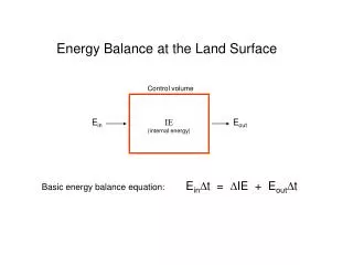
Control volume. E in. IE (internal energy). E out. E in D t = D IE + E out D t. Basic energy balance equation:. Energy Balance at the Land Surface. Energy Balance for a Single Land Surface Slab, Without Snow. S w i + L w i = S w h + L w h + H + l E + C p D T + miscellaneous.


E in
E N D
Presentation Transcript
Control volume Ein IE (internal energy) Eout EinDt = DIE + EoutDt Basic energy balance equation: Energy Balance at the Land Surface
Energy Balance for a Single Land Surface Slab, Without Snow Swi + Lwi = Swh + Lwh + H +lE + CpDT + miscellaneous Terms on LHS come from the climate model. Strongly dependent on cloudiness, water vapor, etc. Terms on RHS come are determined by the land surface model. Sw Sw Lw Lw H lE T where Swi = Incoming shortwave radiation Lwi = Downward longwave radiation Swh = Reflected shortwave radiation Lwh = Upward longwave radiation H = Sensible heat flux l = latent heat of vaporization E = Evaporation rate Cp = Heat capacity of surface slab DT = Change in slab’s temperature, over the time step miscellaneous = energy associated with soil water freezing, plant chemical energy, heat content of precipitation, etc.
Reflected Shortwave Radiation # bands # bands Assume: Sw = S Swdirect, band b + S Swdiffuse, band b b=1 b=1 reflectance for spectral band Compute: Sw = S Sw direct, band b a direct, band b + S Sw diffuse, band b a diffuse, band b # bands b=1 # bands b=1 Simplest description: consider only one band (the whole spectrum) and don’t differentiate between diffuse and direct components: Sw = Sw a Typical albedoes (from Houghton): sand .18-.28 grassland .16-.20 green crops .15-.25 forests .14-.20 dense forest .05-.10 fresh snow .75-.95 old snow .40-.60 urban .14-.18 albedo
Upward Longwave Radiation Stefan-Boltzmann law: Lw = e s T4 where e = surface emissivity s = Stefan-Boltzmann constant = 5.67 x 10⁻⁸ W/(m2K4) T = surface temperature (K) Emissivities of natural surfaces tend to be slightly less than 1, and they vary with water content. For simplicity, many models assume e = 1 exactly.
r cp (Ts - Tr) ra Sensible heat flux (H) Spatial transfer of the “jiggly-ness” of molecules, as represented by temperature Equation commonly used in climate models: H = r cp CH |V| (Ts - Tr), where r = mean air density cp = specific heat of air, constant pressure CH = exchange coefficient for heat |V| = wind speed at reference level Ts = surface temperature Tr = air temperature at reference level (e.g., lowest GCM grid box) For convenience, we can write this in terms of the aerodynamic resistance, ra: H = where ra = 1/ (CH |V|)
V1 R r cp (Ts - Tr) V2 ra H= Why is this form convenient? Because it allows the use of the Ohm’s law analogy: Tr Sensible heat flux ra Electric Current Ts r cp (Ts - Tr) Current = Voltage difference / Resistance I = (V2 – V1) / R H= ra
The aerodynamic resistance, ra, represents the difficulty with which heat (jiggliness of molecules) can be transferred through the near surface air. This difference is strongly dependent on wind speed, roughness length, and buoyancy, which itself varies with temperature difference: 10000 r cp (Ts - Tr) H = 1000 ra ra (s/m) 100 10 1 -10 0 10 Ts - Tr Idealized picture
LATENT HEAT FLUX: The energy used to tranform liquid (or solid) water into water vapor. Latent heat flux from a liquid surface: lvE, where E = evaporation rate (flux of water molecules away from surface) lv = latent heat of vaporization = (approximately) (2.501 - .002361T)106 J/kg Latent heat flux from an ice surface: lsE, where ls = latent heat of sublimation = lv + lm lm = latent heat of melting = 3.34 x 10⁵ J/kg For the purpose of this class, lv and lv will both be assumed constant. We can then discuss the latent heat flux calculation in terms of the evaporation calculation.
Now, some definitions. es(T) = saturation vapor pressure: the vapor pressure at which the condensation vapor onto a surface is equal to the upward flux of vapor from the surface. Clausius-Clapeyron equation: es(T) varies as exp(-0.622 ) Useful approximate equation: es(T) = exp(21.18123 – 5418/T)/0.622, where T is the temperature in oK. l RdT
Specific humidity, q: Mass of vapor per mass of air qr = 0.622 er /p (p = surface pressure, er = vapor pressure) Dewpoint temperature, Tdew: temperature to which air must be reduced to begin condensation. Relative humidity, h: The ratio of the amount of water vapor in the atmosphere to the maximum amount the atmosphere can hold at that temperature. Note: h = er/ es(Tr) = es(Tdew)/ es(Tr) = qs(Tdew)/ qs(Tr) Potential Evaporation, Ep: The evaporative flux from an idealized, extensive free water surface under existing atmospheric conditions. “The evaporative demand”. Four evaporation components Transpiration: The flux of moisture drawn out of the soil and then released into the atmosphere by plants. Bare soil evaporation: Evaporation of soil moisture without help from plants. Interception loss: Evaporation of rainwater that sits on leaves and ground litter without ever entering the soil Snow evaporation: sublimation from the surface of the snowpack
0.622r es(Ts) - er Ep = p ra er Evaporative flux ra es(Ts) The Penman equation can be shown to be equivalent to the following equation, which lies at the heart of the potential evaporation calculation used in many climate models: vapor pressure at reference level =es(Tdew) Note: the ra used here is that same as that used in the sensible heat equation. Does that make sense?
Stomatal resistance is not easy to quantify. rs varies with: -- plant type and age -- photosynthetically active radiation (PAR) -- soil moisture (w) -- ambient temperature (Ta) -- vapor pressure deficit (VPD) -- ambient carbon dioxide concentrations Effective rs for a full canopy (i.e., rc) varies with leaf density, greenness fraction, leaf distribution, etc. rc is essentially a spatially integrated version of rs . Modeling stomatal resistance: “Jarvis-type” models: rs = rs-unstressed(PAR) f1(w)f2(Ta)f3(VPD) Many newer models: rs = f(photosynthesis physics) Key point: Because plants close their stomata during times of environmental stress, rs is modeled so that it increases during times of environmental stress.
Typical approaches to modeling latent heat flux (summary) Transpiration 0.622lr es(Ts) - er lvE = p ra + rs Evaporation from bare soil 0.622lvr es(Ts) - er lvE = p ra + rsurface Resistance to evaporation imposed by soil Interception loss 0.622lvr es(Ts) - er lvE = p ra Note: more complicated forms are possible, e.g., inclusion (in series) of a subcanopy aerodynamic resistance. Snow evaporation 0.622lsr es(Ts) - er lsE = p ra
Bowen Ratio, B: The ratio of sensible heat flux to latent heat flux. Evaporative Fraction, EF: The ratio of the latent heat flux to the net radiative energy. Over long averaging periods, for which the net heating of the ground is approximately zero, these two fractions are simply related: EF = 1/(1+B). Maximum B is infinity (deserts). Minimum EF is 0 (deserts). Minimum B could be close to zero, maximum EF could be close to 1 (rain forests).
HEAT FLUX INTO THE SOIL One layer soil model: Let G be the residual energy flux at the land surface, i.e., G = Sw + Lw - Sw - Lw - H - lE Then the temperature of the soil, Ts, must change by DTs so that G = CpDTs/dt where Cp is the heat capacity dt is the time step length (s)
time of day time of day The choice of the heat capacity can have a major impact on the surface energy balance. Low heat capacity case High heat capacity case -- Heat capacity might, for example, be chosen so that it represents the depth to which the diurnal temperature wave is felt in the soil. -- Note that heat capacity increases with water content. Incorporating this effect correctly can complicate your energy balance calculations.
T1 G12 Internal energy T2 G23 T3 Heat Flux Between Soil Layers One simple approach: G12 = L (T1 - T2) / Dz where L = thermal conductivity Dz = distance between centers of soil layers. Dz temperature -- Using multiple layers rather than a single layer allows the temperature of the surface layer (which controls fluxes) to be more accurate. -- Like heat capacity, thermal conductivity increases with water content. Accounting for this is comparatively easy. depth
Energy balance in snowpack Sw Sw Lw Lw H lsE Internal energy Tsnow lmM GS1 T1 Snow modeling: Plenty of “If statements” Albedo is high when the snow is fresh, but it decreases as the snow ages. Snowmelt occurs only when snow temperature reaches 273.16oK. Internal energy a function of snow amount, snow temperature, and liquid water retention Thermal conductivity within snow pack varies with snow age. It increases with snow density (compaction over time) and with liquid water retention. 1 Solid fraction 0 Temperature 273.16
250oK 260oK Temperature profile snow 270oK 272oK soil Critical property of snow: Low thermal conductivity strong insulation To capture such properties, the snow can be modeled as a series of layers, each with its own temperature. snow soil
Water Balance for a Single Land Surface Slab, Without Snow(e.g., standard bucket model) Terms on LHS come from the climate model. Strongly dependent on cloudiness, water vapor, etc. Terms on RHS come are determined by the land surface model. P = E + R + CwDw/Dt + miscellaneous P E R w where P = Precipitation E = Evaporation R = Runoff (effectively consisting of surface runoff and baseflow) Cw = Water holding capacity of surface slab Dw = Change in the degree of saturation of the surface slab Dt = time step length miscellaneous = conversion to plant sugars, human consumption, etc.
Precipitation, P Getting the land surface hydrology right in a climate model is difficult largely because of the precipitation term. At least three aspects of precipitation must be handled accurately: a. Spatially-averaged precipitation amounts (along with annual means and seasonal totals) b. Subgrid distribution. c. Temporal variability and temporal correlations. Otherwise, even with a perfect land surface model, Perfect land surface model Garbage in Garbage out
Precipitation: subgrid variability (1) The bottom storm is more evenly distributed over the catchment than the top storm. Intuitively, the top storm will produce more runoff, even though the average storm depth over the catchment (E(Yo)) is smaller. Key points: -- Specifying subgrid variability of precipitation is critical to an accurate modeling of surface hydrology. -- A GCM is typically unable to specify the spatial structure of a given storm. The LSM typically has to “guess” it. From Fennessey, Eagleson, Qinliang, and Rodriguez-Iturbe, 1986.
Precipitation: subgrid variability (2) Here, the two storms have similar spatial structure and total precipitation amounts. The locations of the storms, however, are different. If the top storm fell on more mountainous terrain than the bottom storm, the top storm might produce more runoff Key point: A GCM is typically unable to specify the subgrid location of a given storm. The LSM typically has to “guess” it. From Fennessey, Eagleson, Qinliang, and Rodriguez-Iturbe, 1986.
time step 2 time step 3 time step 1 Case 1: No temporal correlation in storm position -- the storm is placed randomly with the grid cell at each time step. Case 2: Strong temporal correlation in storm position between time steps. Precipitation: temporal correlations Temporal correlations are very important -- but are largely ignored -- in GCM formulations that assume subgrid precipitation distributions. This is especially true when the time step for the land calculation is of the order of minutes. Why are temporal correlations important? Consider three consecutive time steps at a GCM land surface grid cell: Case 2 should produce, for example, stronger runoff.
Throughfall Simplest approach: represent the interception reservoir as a bucket that gets filled during precipitation events and emptied during subsequent evaporation. Throughfall occurs when the precipitation water “spills over” the top of the bucket. Capacity of bucket is typically a function of leaf area index, a measure of how many leaves are present. This works, but because it ignores subgrid precipitation variability (e.g., fractional wetting), it is overly simple.
Spatial precipitation variability and interception loss SiB’s approach (Seller’s et al, 1986) Precipitation assumed to fall according to some prescribed distribution Area above line is considered throughfall Capacity of reservoir Note: SiB allows some of the precipitation to fall to the ground without touching the canopy. Original water in reservoir
Temporal precipitation variability and interception loss Mosaic LSM’s approach:
Runoff a. Overland flow: (i) flow generated over permanently saturated zones near a river channel system: “Dunne” runoff (ii) flow generated because precipitation rate exceeds the infiltration capacity of the soil (a function of soil permeability, soil water content, etc.): “Hortonian” runoff b. Interflow (rapid lateral subsurface flow through macropores and seepage zones in the soil c. Baseflow (return flow to stream system from groundwater) Runoff (streamflow) is affected by such things as: -- Spatial and temporal distributions of precipitation -- Evaporation sinks -- Infiltration characteristics of the soil -- Watershed topography -- Presence of lakes and reservoirs
Modeling runoff: GCM scale Surface runoff formulations in GCMs are generally very crude, for at least two reasons: (i) Developers of GCM precipitation schemes have focused on producing accurate precipitation means, not on producing accurate subgrid spatial and temporal variability. (ii) GCM land surface models generally represent the hydrological state of the grid cell with grid-cell average soil moistures -- the time evolution of subgrid soil moisture distributions is not monitored. At best, we can expect first-order success with these runoff formulations
Soil Moisture Transport, Baseflow First, some useful definitions: Porosity (n): The ratio of the volume of pore space in the soil to the total volume of the soil. When a soil with a porosity of 0.5 is completely dry, it is 50% rock by volume and 50% air by volume. Volumetric moisture content (q): The ratio of the volume of water in the soil to the total volume of soil. When the soil is fully saturated, q = n. Degree of saturation (w): The ratio of the volume of water in the soil to the volume of water at saturation. By definition, w= q /n. Pressure head (y): A measure of the degree to which the soil holds on to its water through tension forces. More specifically, y =p/rg, where r is the density of water, g is gravitational acceleration, and p is the fluid pressure. Elevation head (z): The height of soil element above an arbitrary baseline. Hydraulic head (h): The sum of the pressure head and the elevation head. Wilting point: The soil moisture content (measured either in degree of saturation or pressure head) at which plants can no longer draw the moisture from the soil. When modeling the root zone, this is often considered to be the lowest moisture content possible. Field capacity: The water content obtained when a saturated soil drains to the point where the surface tension on the soil particles balances the gravitational forces causing drainage.
L h2 h1 Estimating water transport in the saturated zone (i.e., below water table) Darcy’s Law states that Q/A = flow per unit normal area = - K where K = hydraulic conductivity h = hydraulic head L = separation distance h2 - h1 L More generally, q = - K h q = specific discharge = Q/A Generalized Darcy’s Law: relates flow to gravitational and pressure forces. (Recall: h = y + z)
krg K = m Hydraulic conductivity, K, is related to the soil’s specific permability: Where r is the fluid’s density and m is its dynamic viscosity. K is thus a function of soil and fluid properties. K varies tremendously with soil type. Small variations in soil type, say across a field site, could lead to orders of magnitude difference in the ability to transport moisture. From Freeze and Cherry
y(w) = ysaturated w -b K(w) = Ksaturated w 2b+3 b = empirical coefficient Unsaturated zone equations (from Clapp and Hornberger) Moisture transport in the unsaturated zone (e.g., in the soil near the surface) can also be computed with Darcy’s law, if appropriate corrections are made to pressure head and hydraulic conductivity. qr = residual moisture “specific retention” Z If atmospheric pressure defined to be 0. qr Recall: q = ratio of water volume to soil volume, n = porosity Soil moisture profile capillary fringe p < 0 p = 0 q=n q p > 0 Water table Recall: w= degree of saturation, = q/n
w1 d1 surface layer w2 d2 root layer d3 w3 recharge layer One possible discretization of Darcy’s law (continued) Characterize the soil as stacked layers (d = thickness) Compute for each layer i: yi = ysat wi-b Ki = Ksat wi 2b+3 Compute flow from layer i to layer i+1: yi - yi+1 qz i,i+1 = K + 1 d K = “average” K across distance = (diKi + di+1Ki+1)/(di+di+1) d = effective depth for computing gradient = 0.5 (di+di+1) For drainage out the bottom of the soil column (QD), one might equate it to the hydraulic conductivity in the lowest layer. SiB, for example, goes beyond this by also applying a “mean slope angle” term, sin x: QD = K3 sin x
Energy balance versus water balance Water balance: Implicit solution usually not necessary Results in updated water storage prognostics Energy balance: Implicit solution usually necessary Results in updated temperature prognostics How are the energy and water budgets connected? 1. Evaporation appears in both. 2. Albedo varies with soil moisture content. 3. Thermal conductivity varies with soil moisture content. 4. Thermal emissivity varies with soil moisture content. Question: Can we address how the energy and water budgets together control evaporation rates?
Budyko’s analysis of energy and water controls over evaporation These assymptotes act as barriers to evaporation.
What determines the shape of Budyko’s curve? If only annual means mattered, the observed curve should look like this:
Note that if these seasonal effects alone were considered, the observed curve would actually look like this:
This effect can bring the curve in line with the observed curve. Note, though, that other effects also contribute to a region’s evaporation rate, including land surface properties and the temporal variation of precipitation.
Budyko’s analysis: discussion 1. Annual precipitation and net radiation control, to first order, annual evaporation rates. 2. The spread of points around the Budyko curve is large, though, due to various additional factors: -- phasing of seasonal P and Rnet cycles -- interseasonal storage of moisture -- Other land surface or meteorological effects (vegetation type and resistance, topography, rainfall statistics, …) 3. Note also: -- Land surface processes affect the precipitation and net radiation forcing -- there’s not truly a clean separation between land and atmospheric effects. -- The land’s effects on hourly, daily and monthly evaporation are relatively much more important than they are on annual evaporation.
Structure of a Mosaic LSM tile: Water Balance precipitation evaporation + transpiration INTERCEPTION RESERVOIR throughfall surface runoff infiltration SURFACE LAYER ROOT ZONE LAYER soil moisture diffusion RECHARGE LAYER drainage
GCM P, radiation, Tair, etc. E, H, upward longwave LSM How do we evaluate the performance of such an LSM? “Online” approach: test GCM output against observations. Advantage: The coupling effects can be studied, and various sensitivity tests can be performed. Disadvantage: The model forcing (precipitation, radiation, etc.) can be wrong, so validating the land surface model can be very difficult. (“Garbage in -- Garbage out”) Example from GISS GCM/LSM: The Amazon river is poorly simulated, but we can’t tell if this is due to a bad LSM or poor precipitation from the GCM.
Better approach: Offline forcing (one-way coupling) Forcing Data Advantage: Land surface model can be driven with realistic atmospheric forcing, so that the impact of the LSM’s formulations on the surface fluxes can be isolated. Disadvantage: Deficient behavior of the LSM may seem small in offline tests but may grow (through feedback) in a coupled system. Thus, offline tests can’t get at all of the important aspects of a land surface model’s behavior. Output File P, radiation, Tair, etc. E, H, Rlw , diagnostics LSM PILPS model intercomparisons (to be discussed in a later lecture) have largely focused on such offline evaluations.
DYNAMIC VEGATION: Yet another step forward in model development Typical GCM approach: ignore effects of climate variations on vegetation Early attempts at accounting for vegetation/ climate consistency Fully integrated dynamic vegetation model Figure from Foley et al., “Coupling dynamic models of climate and vegetation”, Global Change Biology, 4, 561-579, 1998.
as described by bT and fR Thus, it is the relative positions of the runoff and evaporation functions that determine the annual transpiration rate -- not the average soil moisture. Most important take-home lesson: soil moisture in one model need not have the same “meaning” as that in another model. As long as the transpiration and runoff curves have the same relative positions, two models (e.g., Models A and B below) will behave identically, even if they have different soil moisture ranges. (True for simple models in simple water balance framework and for complex LSMs running in AGCMs.) Model A Model B 1 1 bT bT R R 0 0 0 200 400 600 800 1000 0 200 400 600 800 1000
Sure enough, the LSMs in PILPS have different soil moisture ranges... …and there is no evidence that LSMs with higher soil moistures produce higher evaporations.
Important aside: What does “model-produced soil moisture” mean? What are the implications of a misinterpreted soil moisture? Common problem: GCM “A” needs to initialize its land model with realistic soil moistures for some application (e.g., a forecast). Misguided, dangerous, and all too common solution: Use soil moistures generated by GCM “B” during a reanalysis or by land model “C” in an offline forcing exercise (e.g., GSWP), after correcting for differences in layer depths and possibly soil type. This solution is popular because of a misconception of what “soil moisture” means in a land model. Contrary to popular belief, -- model “soil moisture” is not a physical quantity that can be directly measured in the field. -- model “soil moisture” isbest thought of as a model- specific “index of wetness” that increases during wet periods and decreases during dry periods.
Should a land modeler be concerned that modeled soil moisture has a nebulous meaning – that it doesn’t match observations? It depends on one’s outlook.Consider that in the real world: (1) soil moisture varies tremendously across the distances represented by GCM grid cells, (2) surface fluxes (evaporation, runoff, etc.) vary nonlinearly with soil moisture. and dry evaporation efficiency wet wet hundreds of km soil moisture