Download

1 / 33
350 likes | 373 Views
Explore the physics of air-surface interactions and coupling to ocean/atmosphere processes, emphasizing surface fluxes. Delve into the history and present status of surface flux parameterizations, including turbulent fluxes and CO2 flux measurements. Investigate gas and particle fluxes, addressing parameterization challenges in global climate models.

E N D
Air-Sea Interaction:Physics of air-surface interactions and coupling to ocean/atmosphere BL processes • Emphasize surface fluxes • Statement of problem • Present status • Parameterization issues • An amusing case
Present Status of Surface Flux Parameterizations • P: No dependence on surface variables • Radiation: Depends on albedo, emissivity, and Ts but real problem is clouds • Turbulent Fluxes: Bulk Parameterization
Physically-Based Parameterizations Old Days: CE=1E-3 and k=0.003*U2 and spray=S(r)*fwhitecap
Historical perspective on turbulent fluxes:Typical moisture transfer coefficients Algorithms of UA (solid lines), COARE 2.5 (dotted lines), CCM3 (short-dashed lines), ECMWF (dot-dashed lines), NCEP (tripledot-dashed lines), and GEOS (long-dashed lines) .
Air-Sea transfer coefficients as a function of wind speed: latent heat flux (upper panel) and momentum flux (lower panel). The red line is the COARE algorithm version 3.0; the circles are the average of direct flux measurements from 12 ETL cruises (1990-1999); the dashed line the original NCEP model.
CO2 Flux: Transfer velocity versus wind speedHare, McGillis, Edson, Fairall Work under way on DMS and Ozone
Particle Fluxes • Optically relevant (.1 – 10 micron): • Principally whitecap-bubble production • Measurement and interpretation problems • Some dependence on laboratory work • No consensus • Thermodynamically relevant (50-500 micron) • Principally breaking-wave spume production • No measurements at high winds • Order of magnitude uncertainty
Progress in Last 5ish Years • Conventional turbulent fluxes: • Greatly expanded data base • 5% 0-20 m/s • Progress on wind-wave-stress models • M-O stability functions, light-wind convective & stable • Gas Fluxes: • Ship-based covariance measurements • Physically-based parameterization • Particle Fluxes: • Expanded modeling efforts
Flux Parameterization Issues • Representation in GCM • Except for P, most observations are point time averages • Concept of gustiness sufficient? • Mesoscale variable? Precip, convective mass flux, … • Strong winds • General question of turbulent fluxes, flow separation, wave momentum input • Sea spray influence • Waves • Stress vector vs wind vector (2-D wave spectrum) • zo vs wave age & wave height • Breaking waves • Gas and particle fluxes • Distribution of stress and TKE in ocean mixed layer (P. Sullivan) • Gas fluxes • Bubbles • Surfactants (physical vs chemical effects) • Extend models to chemical reactions • Particle fluxes • Interpretation of measurements • Source vs deposition
Strong wind turbulent fluxes • Direct turbulent fluxes • Cd or Charnock coeff • Ch/Ce or zot/zoq=f(Rr) • Droplet mediated fluxes • Momentum <ρwu> • Mass flux <ρw> • Enthalpy flux; partitioning Qs and Ql
Evidence • Strom surge models • Cd/Ck ratio, Emanuel • Powell drop sonde profiles • Price ocean mixed layer integrations • Laboratory simulations Explanations Slippery young waves (direct Cd) – Moon et al Droplet mass effect (ρ<w’u’>– Andreas Droplet stability effect (<w’ ρ’> - Makin
GOES SST imagery. Daily composites made from hourly images. GOES seems • to be the most prolific SST imaging system, though at the expense of accuracy and • noise level. • SST cooling in these images exhibits: • Significant horizontal structure, i) a marked rightward bias, ii) along-track • variability that is not correlated with intensity, and, • 2) A rapid relaxation back toward pre-storm SST, e-folding approx 10 days. day 250 EM-APEX 1634 1633 1636
A numerical simulation of the UO response The numerical ocean model is Price et al., '94; grid-level, high resolution, closed with PWP upper ocean mixing algorithm. The ocean IC is from pre-Frances EM-APEX. The single most important thing is the hurricane stress field: a fit to HWINDS for the wind field and Powell et al. for the drag coefficient. The implicit assumption is that stressocean= stressairand so this is the null model with respect to some of the most interesting effects of surface waves.
A Sea-Spray Thermodynamic Parameterization Including Feedback C. W. Fairall *, J-W. Bao, and J. WilczakNOAA Environmental Technology Laboratory (ETL)Boulder, CO • Background • Source strength • Feedback • Sensitivities • Model tests
Droplet Source Functions Fairall et al. 1994 Fairall, Banner, Asher Physical Model P energy wave breaking σ surface tension r droplet radius η Kolmogorov microscale f fraction of P going into droplet production Vf=droplet mean fall velocity
Partitioning of Droplet Contribution:Stages of cooling/evaporation • Simplification: consider large droplets that are ejected, cool to wet bulb temperature and re-enter ocean with negligible change in mass • Stages: • Cool from To to Tair = Qs • Cool from Tair to Twet = Ql_a • Evaporation while at Twet = Ql_b • Total droplet enthapy transfer Qse=Qs+Ql_a • Enthalpy Bowen ratio = Qs/Ql_a=(To-Ta)/(Ta-Twet) • Qs=Qse*bowen/(1+bowen)
Feedback Characterization δTa Effect on the fluxes:
Model Tests (Bao and Ginis) • IVAN, ISABEL • GFDL operational • GFDL new zo, zt • WRF • PLANS • HWRF at high resolution – matrix of tune values • Explicit droplet model (Kepert/ Fairall) in HWRF • Coordinate with Penn State LES work
But:Simulations with New Cd and Ce/Ch Old Cd Ce/Ch New Cd Ce/Ch