Advanced 2-Way Time Forward Modeling for Diffraction Stack and Reflectivity Analysis
This document explores advanced techniques in forward modeling within the context of diffraction stack and reflectivity analysis. We detail the mathematical framework including Green's functions, asymptotic approximations, and Fourier transforms to accurately simulate wave propagation in subsurface imaging. The modeling incorporates multiple reflector types and varying wavelet energy distributions. MATLAB exercises are provided for practical application, allowing the generation of synthetic data based on various geological models. This comprehensive approach enhances understanding of subsurface characteristics through accurate simulation methodologies.


Advanced 2-Way Time Forward Modeling for Diffraction Stack and Reflectivity Analysis
E N D
Presentation Transcript
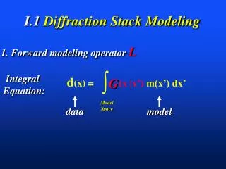
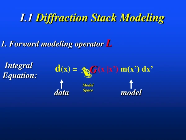
d(x) = (x |x’) m(x’) dx’ G Integral Equation: ò model data Model Space I.1 Diffraction Stack Modeling 1. Forward modeling operator L
2-way time Forward Modeling
2-way time Forward Modeling: Sum of Weighted Hyperbolas
iw|x-x’|/c Phase e |x-x’| Geom. Spread |x-x’| x x’ GREEN’s FUNCTION G(x|x’) =
iw|x-x’|/c Phase xx’ xx’ e -1 + O( ) |x-x’| Geom. Spread x x’ ASYMPTOTIC GREEN’s FUNCTION G(x|x’) = A(x,x’)
i xx’ R(x’) x’ x’ reflectivity ASYMPTOTIC GREEN’s FUNCTION e G(x|x’) = A(x,x’)
1-way time Diffraction Stack Modeling = ZO Modeling
2-way time Diffraction Stack Modeling = ZO Modeling Dipping Reflector
1-way time Diffraction Stack Modeling = ZO Modeling If c for DS is ½ that for ZO Modeling
i i xx’ xx’ R(x’) x’ x’ reflectivity Fourier Transform: F e (t- ) xx’ (t- ) ~ F xx’ d(x) R(x’) A(x,x’) ASYMPTOTIC GREEN’s FUNCTION ~ e d(x) = A(x,x’)
QUICK REVIEW FOURIER TRANSFORM ( - t) xx’ i e d t Cos( 4 t ) + + (t- ) Cos( 2 t ) xx’ + Cos( 3 t ) cancellation cancellation Cos( t ) constructive reinforcement @ t=0 (t)
x’ time Sum over reflectivity Spray energy along hyperbolas (t- ) xx’ (t- ) xx’ Forward Modeling Operator d(x,t) = R(x’) A(x,x’)
W x’ time CANCELLATION REINFORCE (t- ) xx’ Forward Modeling Operator d(x,t) = R(x’) A(x,x’)
SUMMARY x’ d(x) = (x |x’)m(x’) dx’ G Integral Equation: reflectivity ò Source wavelet Geom. spreading model data Model Space W (t- ) xx’ 1. Exploding Reflector Modeling = Diffraction Stack Modeling R(x’) d(x,t) = Sum over reflectors Data variables A(x,x’) 2. High Frequency Approximation (i.e c(x) variations > 3* ) 3. Approximates Kinematics of ZO Sections, but not Dynamics
x’ d(x,t|x’,0) = R(x’) W (t- ) xx’ MATLAB Exercise: Forward Modeling 1. To account for the source wavelet W(t), we convolve data with W(t)(recall (t- )*W(t)= W() ) so that modeling equation becomes (neglect A) A). Execute MATLAB program forw.m to generate synthetic data for a point scatterer and a 30 Hz wavelet. B). Execute MATLAB program forwl.m to generate synthetic data for a dipping layer model C). Execute MATLAB program forw.m to generate synthetic data for a syncline model. Note diffractions and multiple arrivals. Adjust for new models. Why the second time derivative?
x’ d(x,t) = R(x’) Loop over traces Loop over x in model Loop over z in model Traveltime { W (t- ) R(x’) xx’ MATLAB Exercise: Forward Modeling for ixtrace=1:ntrace; for ixs=istart:iend; for izs=1:nz; r = sqrt((ixtrace*dx-ixs*dx)^2+(izs*dx)^2); time = 1 + round( r/c/dt ); data(ixtrace,time) = migi(ixs,izs)/r + data(ixtrace,time); end; end; data1(ixtrace,:)=conv2(data(ixtrace,:),rick); end; * Src Wave