Download

1 / 43
430 likes | 466 Views
Explore the latest advancements in the Particulate Inorganic Carbon (PIC) algorithm for ocean studies, cross-platform comparisons, and application of Collection 6 data from SeaWiFS and MODIS. Discover insights on PIC variability and its implications on global turnover.

E N D
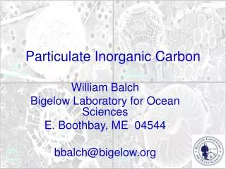
Particulate Inorganic Carbon William Balch Bigelow Laboratory for Ocean Sciences E. Boothbay, ME 04544 bbalch@bigelow.org
Acknowledgments • Bruce Bowler, Dave Drapeau and Laura Lubelczyk, (Bigelow Laboratory for Ocean Sciences) • Captains and crew of: RRS Discovery, R/V Melville, R/V Revelle, R/V Ron Brown, RRS James Clark Ross, RRS James Cook, R/V Thompson; R/V Tangaroa; M/S Scotia Prince; M/S The CAT • Norman Kuring- NASA Goddard • Goddard Ocean Color Group • Giovanni and Ocean Data View • NASA support
PIC algorithm is typically focused on coccolithophores- ubiquitous, single-cell calcifying plants There are other PIC particles in the sea but coccoliths and coccolithophores have the highest scattering per unit PIC (“backscattering cross section”)
A B E. huxleyi Ophiaster sp. C D Calcidiscus leptoporous Papposphaera sp. Outline • PIC algorithm cross platform comparisons • PIC algorithm refinement • Science applications
Cross platform algorithm variability • SeaWiFS • MODIS Terra • MODIS Aqua
Merged Two-Band/Three band algorithm for PIC applied to SeaWiFS and MODIS-Aqua data (Collection 6)…Similar patterns
PIC Algorithm Performance: Collection 6 SeaWiFS PIC (9km; mol m-3) MODIS Aqua PIC (9km; mol m-3) Linear Scales
Aqua PIC (9km; mol m-3) SeaWiFS Aqua PIC (9km; mol m-3) PIC Algorithm Performance: Collection 6 MODIS Aqua PIC, on average, < SeaWiFS Apic = 0.87228*Spic + 3.6902e-5r^2 = 0.8125DF = 2,965,214SEy = 6.7025e-4Fstat = 1.2851e+7 RMSe = 0.001547 (y) Log Scales
Subtropics Temperate and sub polar Summer blooms Collection 6; 2002-2010; global MODIS AQUA Frequency (x105) -4 -3 -2 -1 SeaWiFS Frequency (x106) -4 -3 -2 -1 Log PIC (mol m-3)
We’ve used MISR to measure coccolith backscattering… using the Blue bands, integrated -70o to 70o, subtracting the NIR band (quasi atmosphere correction), then a dark pixel assumption to further correct.
PIC algorithm refinement • The backscattering that we associated with chlorophyll has been adjusted for PIC. • The backscattering cross section of PIC (bb*; m2 mol-1) has been adjusted (based on cruise work). Variable bb* algorithm. • New K490 formulation in PIC algorithm (formerly Baker and Smith 1982; now Morel and Martorena, 2001) • Fo has been updated to what is used in SeaDAS
Many major cruises to study coccolithophores- both northern and southern hemisphere; sampled over >212,000 km… Arctic’11 GNATS’98-’12 AMT 15-22 SW Pacific’11 Tangaroa Great Belt ’12 Great Belt ’11 SOGasEx’10 Patagonian Shelf’08
Mean bb PIC bbp (m-1) All data points are bbp acid (no PIC)
Current New LUT changes bb PIC (m-1) 5 4 3 2 1 0 0.020 0.015 0.010 0.005 0.000 nLw550 0 1 2 3 4 5 6 7 8 9 10 nLw443
Compass (earlier version) Satlantic Micro-SAS radiometers collect along-track data for Lt, Lsky, and Ed. We designed a mount which compensated real-time for changes in sun’s azimuth relative to ship heading. Radiometers mounted on the RRS Discovery Balch; Bigelow Lab
New LUT Old LUT Algorithm improvement (n=~800)
Relating Surface to integrated PIC… Integral > expected if homogenously dist. Integrated PIC (to 100m depth; mmol m-2) Integral < expected if homogenous dist. The more surface PIC, the more likely it is confined to the surface layer Surface PIC (mmol L-1)
+ + + + + + + + Using MODIS SST, Aquarius SSS to define global surface density field. High PIC sits at the strong gradients of Sub Antarctic Frontal boundary
PIC (mol m-3) 0.01 0.003 0.001 0.0003 0.0001 0.00003 Plot surface PIC concentration in temperature/salinity space Isopleths of density; sigma theta PIC (Dec’12) 18 30 25 20 15 10 5 0 19 20 21 22 27 28 Temperature (oC) 23 29 24 30 25 26 31 30 31 32 33 34 35 36 37 38 39 Salinity
PIC Global Time Series (MODIS-Aqua)Mission record Integrated Global PIC (top 100m; moles PIC) Fraction of Maximum Value Date
PIC Global Time Series (MODIS-Aqua)Annual coccolithophore phenology
PIC Global Time Series (MODIS-Aqua)Annual coccolithophore phenology
Implications of these results to PIC turnover… • Average global PIC =~5[+/-1] x 1011 moles PIC =6 x 10¹² g PIC • Global calcification = 1.6[+/-0.3] Pg PIC y-1 Balch et al., 2007 • (6 x 10¹² g PIC)/(1.6 x 1015 g PIC y-1)= 0.003 y =~1.1d turnover • What is happening to it? It sinks or dissolves • No indication of a trend in global PIC (e.g. negative trend associated with OA)
Summary- PIC algorithm • Cross platform comparisons of PIC are within 3-13% depending on the platform • MISR can be used to detect coccolithophores • New improved PIC algorithm has accuracy of +/-0.2-0.3mmol PIC m-3= 2-3mg PIC L-1 • PIC is not homogenously distributed but shows subsurface maxima in oligotrophic waters, and surface maxima in blooms; use this to improve vertical integrations based on surface PIC estimates
Summary- Science Issues • Highest [PIC] seen globally at frontal boundaries between surface seawater densities (sq) 26-27 (SSS 34-36 and SST 2-15oC) • Greatest global PIC standing stock in January and lowest in March • Global phenology of coccolithophore blooms shows greatest average [PIC] associated with austral summer, boreal summer lower, lowest at the equinoxes
Future tasks at hand; Improve PIC algorithm performance • Examine using reflectance-differencing algorithm (Hu et al., 2012) for determining bb chl • Improve predictions of global variability of bb* • Partition backscattering into bb POC, bb PIC and bb BSi
Future: MODIS Science • Examine coccolithophore bloom at sub-kilometer pixel resolution using MISR and high-resolution land bands. What can we learn about processes driving bloom at these scales? • Examine global coccolithophore phenologyin different portions of world ocean (different biogeochemical provinces) • Frontal impacts on coccolithophore growth (using Aquarius salinity; MODIS SST)
Future: MODIS Science • Impact of wind speed on coccolithophore standing stocks (AMSR-E or Aquarius winds) • Examine PIC Turnover in different regions of world as foci for ballasted sinking POC • Are there long-term negative trends of PIC associated with Ocean Acidification, especially in polar provinces where OA will have biggest effects?
A B E. huxleyi Ophiaster sp. C D Calcidiscus leptoporous Papposphaera sp. Thank you!
While satellites generally agree with collection 6, shipboard validation data show underestimates...the issue is bb* Sampled within ½ h of overpass
Use shipboard radiance data to predict PIC bb… 10-1 10-2 10-3 10-4 10-5 bbPIC (SAS above water nLw; m-1) 10-5 10-4 10-3 10-2 10-1 bbPIC (ship seawater; m-1)
MODIS Terra PIC, on average, ~6% > MODIS Aqua Aqua Vs TerraTpic = 1.0641*Apic - 1.3028e-5r^2 = 0.8146DF = 2,965,214SEy = 7.8592e-4Fstat = 1.3025e+7RMSe = 0.001825 (y) Terra PIC (9km; mol rm-3) MODIS Aqua PIC (9km; mol m-3)
MODIS Terra, on average, within ~3% of SeaWiFS SeaWiFS vs TerraTpic = 0.97532*Spic + 8.8717E-6r^2 = 0.7308DF = 2,965,214SEy = 9.4698e-4Fstat = 8.0484e+6 RMSe = 0.001825 (y) Terra PIC (9km; mol m-3) SeaWiFS PIC (9km; mol m-3)