Populations

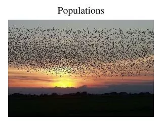
2. Populations • Organisms do not generally live alone. A population is a group of organisms from the same species occupying in the same geographical area. • This area may be difficult to define because: • A population may comprise widely dispersed individuals which come together only infrequently, e.g. for mating. • Populations may fluctuate considerably over time. Migrating wildebeest population Tiger populations comprise widely separated individuals

3. Features of Populations 1 • Populations are dynamic and exhibit attributes that are not shown by the individuals themselves. • These attributes can be measured or calculated and include: • Population size: the total number of organisms in the population. • Population density: the number of organisms per unit area. • Population distribution: the location of individuals within a specific area.

4. Features of Populations 2 • Population composition provides information relevant to the dynamics of the population, i.e. whether the population is increasing or declining. • Information on population composition (or structure) includes: • Sex ratios: the number of organisms of each sex. • Fecundity (fertility): the reproductive capacity of the females. • Age structure: the number of organisms of different ages.

5. Population Dynamics • The study of changes in the size and composition of populations, and the factors influencing these changes, is population dynamics. • Key factors for study include: • Population growth rate: the change in the total population size per unit time. • Natality (birth rate): the numberof individuals born per unit time. • Mortality (death rate): the number of individuals dying per unit time. • Migration: the number moving into or out of the population. Population size is influenced by births… …and deaths

6. Migration • Migration is the movement of organisms into (immigration) and out of (emigration) a population. It affects population attributes such as age and sex structure, as well as the dynamics of a population. • Populations lose individuals through deaths and emigration. • Populations gain individuals through births and immigration. Wildebeest Canada geese Migrating species may group together to form large mobile populations

7. Population Density • The number of individuals per unit area (for terrestrial organisms) or volume (for aquatic organisms) is termed the population density. • At low population densities, individuals are spaced well apart. Examples: territorial, solitary mammalian species such as tigers and plant species in marginal environments. • At high population densities, individuals are crowded together. Examples: colonial animals, such as rabbits, corals, and termites. Low density populations High density populations

8. Population Distribution • A crude measure of population density tells us nothing about the spatial distribution of individuals in the habitat. • The population distribution describes the location of individuals within an area. • Distribution patterns are determined by the habitat patchiness (distribution of resources) and features of the organisms themselves, such as territoriality in animals or autotoxicity in plants. • Individuals in a population may be distributed randomly, uniformly, or in clumps. Clumped distribution in termites More uniform distribution in cacti

9. Random Distribution • A population’s distribution is considered random if the position of each individual is independent of the others. • Random distributions are not common; they can occur only where: • The environment is uniform and resources are equally available throughout the year. • There are no interactions between individuals or interactions produce no patterns of avoidance or attraction. • Random distributions are seen in some invertebrate populations, e.g. spiders and clams, and some trees. Spider populations appear to show a random distribution

10. Uniform Distribution • Uniform or regular distribution patterns occur where individuals are more evenly spaced than would occur by chance. • Regular patterns of distribution result from intraspecific competition amongst members of a population: • Territoriality in a relatively homogeneous environment. • Competition for root and crown space in forest trees or moisture in desert and savanna plants. • Autotoxicity: chemical inhibition of plant seedlings of the same species. Saguaro cacti compete for moisture and show a uniform distribution

11. Clumped Distribution • Clumped distributions are the most common in nature; individuals are clustered together in groups. • Population clusters may occur around a a resource such as food or shelter. • Clumped distributions result from the responses of plants and animals to: • Habitat differences • Daily and seasonal changes in weather and environment • Reproductive patterns • Social behavior Sociality leads to clumped distribution

12. Population Regulation DIRECTLY OR INDIRECTLY AFFECTS FOOD SUPPLY Poor health or death INCREASE IN MORTALITY Change in ability to reproduce NATALITY IS AFFECTED • Population size is regulated by environmental factors that limit population growth. These may be dependent or independent of the population density.

13. Environmental Factors • Environmental factors may be categorized according to how much population density influences their effect on population growth: • Density independent factors have a controlling effect on population size and growth, regardless of the population density. • Density dependent factors have an increasing effect on population growth as the density of the population increases. Severe fires can result in high mortality Humans often live at high density

14. Density Dependent Factors • Density dependent factors exert a greater effect on population growth at higher population densities.At high densities, individuals: • Compete more for resources. • Are more easily located by predators and parasites. • Are more vulnerable to infection and disease. • Density dependent factors are biotic factors such as food supply, disease, parasite infestation, competition, and predation. Competition increases in crowded populations Parasites can spread rapidly through dense populations

15. Density Independent Factors • The effect of density independent factors on a population’s growth is not dependent on that population’s density: • Physical (or abiotic) factors • temperature • precipitation • humidity • acidity • salinity etc. • Catastrophic events • floods and tsunamis • fire • drought • earthquake and eruption

16. Population Growth Population growth = Births – Deaths + Immigration – Emigration (B) (D) (I) (E) • Population growth depends on the number of individuals added to the population from births and immigration, minus the number lost through deaths and emigration. • This can be expressed as a formula: • Net migration is the difference between immigration and emigration.

17. Calculating Population Change Deaths (D) Immigration (I) Births (B) Emigration (E) Births, deaths, and net migrations determine the numbers of individuals in a population

18. Rates of Population Change • Ecologists usually measure the rate of population change. • These rates are influenced by environmental factors and by the characteristics of the organisms themselves. • Rates are expressed as: • Numbers per unit time,e.g. 2000 live births per year • Per capita rate (number per head of population),e.g. 122 live births per 1000 individuals (12.2%) Many invertebrate populations increase rapidly in the right conditions Large mammalian carnivores have a lower innate capacity for increase

19. Exponential Growth Colonizing Population • Populations becoming established in a new area for the first time are often termed colonizing populations. • They may undergo a rapid exponential (logarithmic) increase in numbers to produce a J-shaped growth curve. • In natural populations, population growth rarely continues to increase at an exponential rate. • Factors in the environment, such as available food or space, act to slow population growth. Here the number being added to the population per unit time is large. Exponential (J) curveExponential growth is sustained only when there are no constraints from the environment. Population numbers (N) Here, the number being added to the population per unit time is small. Lag phase Time

20. Logistic Growth • As a population grows, its increase will slow, and it will stabilize at a level that can supported by the environment. • This type of sigmoidal growth produces the logistic growth curve. Established Population Environmental resistance increases as the population overshoots K. The population encounters resistance to exponential growth as it begins to fill up the environment. This is called environmental resistance. Carrying capacity (K) The population density that can be supported by the environment. Logistic (S) curve As the population grows, the rate of population increase slows, reaching an equilibrium level around the carrying capacity. Population numbers (N) Environmental resistance decreases as the population falls below K. The population tends to fluctuate around an 'equilibrium level'. The fluctuations are caused by variations in the birth rate and death rate as a result of the population density exceeding of falling below carrying capacity. In the early phase, growth is exponential (or nearly so) Lag phase Time

21. Life Tables • Numerical data collected during a population study can be presented as a table of figures called a life table. • Lifetables provide a summary of mortality for a population. The basic data are the number of individuals surviving to each age interval. This gives the ages at which most mortality occurs in a population. Life table for a population of the barnacle Balanus

22. Survivorship Curves • The age structure of a population can represented with asurvivorship curve. Survivorship curves use a semi-log plot of the number of individuals surviving per 1000 in the population, against age. • Because they are standardized (as number of survivors per 1000),species with different life expectancies can be easily compared. • The shape of the curve reflects where heaviest mortality occurs: Type I: late loss large mammals Type II: constant loss small mammals, songbirds Number of survivors (log scale) Type III: early loss oysters, barnacles Relative age

23. Type I Survivorship Curves • Species with Type I or late loss survivorship curves show the heaviest mortality late in life. Mortality is very low in the juvenile years and throughout most of adult life. • Late loss curves are typical of species that produce few young and care for them until they reach reproductive age. • Such species are sometimes called K selected species and include elephants, humans, and other large mammals. Mortality is very low in early life Mortality increases rapidly in old age

24. Type II Survivorship Curves • Species with Type II or constant loss survivorship curves show a relatively constant mortality at all life stages. • Constant loss curves are typical of species with intermediate reproductive strategies. Populations face loss from predation and starvation throughout life. • Examples include some many types of songbirds, some annual plants, some lizards, and many small mammals. Constant mortality. No one age class is any more susceptible than any other.

25. Type III Survivorship Curves Population losses are high in early life stages • Species with Type III or early loss survivorship curves show the highest mortality in early life stages, with low mortality for those few individuals reaching a certain age and size. • Early loss curves are typical of species that produce large number of offspring and lack parental care. • Such species are r selected species (opportunists), and include most annual plants, most bony fish (although not mouth brooders), and most marine invertebrates. Mortality is low for the few individuals surviving to old age