Download

1 / 54
540 likes | 667 Views
This presentation discusses an innovative approach to optimize multi-dimensional loops using single-dimension software pipelining (SSP). Traditional multi-dimensional loop scheduling methods face challenges due to resource constraints and complexity. SSP simplifies these challenges by identifying the most profitable loop level for scheduling, reusing resources, and maintaining parallelism. The method adapts a resource-constrained approach to effectively manage dependencies and enhance performance. Key concepts include loop selection, dependence simplification, and dynamic scheduling strategies.

E N D
Single-dimension Software Pipelining for Multi-dimensional Loops Hongbo Rong Zhizhong Tang Alban Douillet Ramaswamy Govindarajan Guang R. Gao Presented by: Hongbo Rong IFIP Tele-seminar June 1, 2004
Introduction • Loops and software pipelining are important • Innermost loops are not enough [Burger&Goodman04] • Billion-transistor architectures tend to have much more parallelism • Previous methods for scheduling multi-dimensional loops are meeting new challenges
<1,0> a <0,0> <0,1> b Motivating Example int U[N1+1][N2+1], V[N1+1][N2+1]; L1: for (i1=0; i1<N1; i1++) { L2: for (i2=0; i2<N2; i2++) { a: U[i1+1][i2]=V[i1][i2]+ U[i1][i2]; b: V[i1][i2+1]=U[i1+1][i2]; } } A strong cycle in the inner loop: No parallelism
<1,0> Loop Interchange Followed by Modulo Scheduling of the Inner Loop <0,1> a <0,0> b • Why not select a better loop to software pipeline? • Which and how?
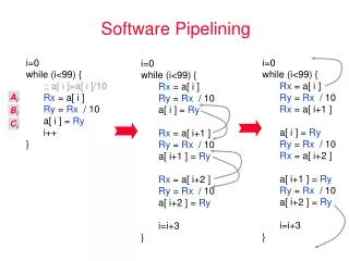
0 1 2 3 4 5 i1 0 1 2 3 4 5 a(0,0) 6 b(0,0) a(1,0) Resource conflicts 7 --- b(1,0) a(2,0) 8 a(0,1) --- b(2,0) a(3,0) 9 <1,0> b(0,1) a(1,1) --- b(3,0) a(4,0) 10 --- b(1,1) a(2,1) --- b(4,0) a(5,0) 11 a a(0,2) --- b(2,1) a(3,1) --- b(5,0) 12 b(0,2) a(1,2) --- b(3,1) a(4,1) --- <0,0> --- b(1,2) a(2,2) --- b(4,1) a(5,1) <0,1> Cycle --- b(2,2) a(3,2) --- b(5,1) --- b(3,2) a(4,2) --- b --- b(4,2) a(5,2) --- b(5,2) --- Starting from A Naïve Approach 2 function unitsa: 1 cycleb: 2 cyclesN2=3
0 1 2 3 4 5 i1 0 1 a(1,0) Kernel, with S=3 stages 2 b(1,0) a(2,0) 3 a(0,1) --- b(2,0) 4 b(0,1) a(1,1) --- 5 --- b(1,1) a(2,1) a(5,0) Slice 1 6 a(0,2) --- a(0,0) b(2,1) a(3,1) b(5,0) Initiation interval T=1 7 b(0,2) a(1,2) b(0,0) --- b(3,1) a(4,1) --- 8 --- b(1,2) --- a(2,2) --- b(4,1) a(5,1) Slice2 9 --- b(2,2) a(3,2) --- a(3,0) b(5,1) 10 --- b(3,2) a(4,2) b(3,0) --- a(4,0) 11 --- b(4,2) --- a(5,2) b(4,0) Slice 3 12 --- b(5,2) --- --- Cycle Looking from Another Angle Resource conflicts
0 1 2 3 4 5 i1 0 1 a(1,0) Kernel, with S=3 stages 2 b(1,0) a(2,0) 3 a(0,1) --- b(2,0) 4 b(0,1) a(1,1) --- 5 --- b(1,1) a(2,1) a(5,0) Delay = (N2-1)*S*T 6 a(0,2) --- a(0,0) b(2,1) a(3,1) b(5,0) Initiation interval T=1 7 b(0,2) a(1,2) b(0,0) --- b(3,1) a(4,1) --- 8 --- b(1,2) --- a(2,2) --- b(4,1) a(5,1) 9 --- b(2,2) a(3,2) --- a(3,0) b(5,1) 10 --- b(3,2) a(4,2) b(3,0) --- a(4,0) 11 --- b(4,2) --- a(5,2) b(4,0) 12 --- b(5,2) --- --- Cycle SSP (Single-dimension Software Pipelining) 7
0 1 2 3 4 5 i1 0 1 a(1,0) Kernel, with S=3 stages 2 b(1,0) a(2,0) a(0,1) 3 --- b(2,0) b(0,1) a(1,1) 4 --- --- b(1,1) a(2,1) 5 a(5,0) Delay = (N2-1)*S*T a(0,2) --- b(2,1) 6 a(0,0) b(5,0) Initiation interval T=1 b(0,2) a(1,2) --- 7 b(0,0) --- --- b(1,2) a(2,2) 8 --- --- b(2,2) 9 a(3,0) --- 10 b(3,0) a(4,0) 11 --- b(4,0) 12 --- Cycle a(3,2) b(3,2) a(4,2) --- b(4,2) --- SSP (Single-dimension Software Pipelining) • An iteration point per cyle • Filling & draining naturally overlapped • Dependences are still respected! • Resources fully used • Data reuse exploited! a(3,1) b(3,1) a(4,1) --- b(4,1) a(5,1) --- b(5,1) --- a(5,2) b(5,2) --- 8
Loop Rewriting int U[N1+1][N2+1], V[N1+1][N2+1]; L1': for (i1=0; i1<N1; i1+=3) { b(i1-1, N2-1) a(i1, 0) b(i1, 0) a(i1+1, 0) b(i1+1, 0) a(i1+2, 0) L2': for (i2=1; i2<N2; i2++) { a(i1, i2) b(i1+2, i2-1) b(i1, i2) a(i1+1, i2) b(i1+1, i2) a(i1+2, i2) } } b(i1-1, N2-1)
Outline • Motivation • Problem Formulation & Perspective • Properties • Extensions • Current and Future work • Code Generation and experiments
Problem Formulation Given a loop nest L composed of n loops L1, …, Ln, identify the most profitable loop level Lx with 1<= x<=n, and software pipeline it. • Which loop to software pipeline? • How to software pipeline the selected loop? • How to handle the n-D dependences? • How to enforce resource constraints? • How can we guarantee that repeating patterns will definitely appear?
Single-dimension Software Pipelining • A resource-constrained scheduling method for loop nests • Can schedule at an arbitrary level • Simplify n-D dependences to 1-D • 3 steps • Loop Selection • Dependence Simplification and 1-D Schedule Construction • Final schedule computation
Enforce resource constraints in two steps Perspective • Which loop to software pipeline? • Most profitable one in terms of parallelism, data reuse, or others • How to software pipeline the selected loop? • Allocate iteration points to slices • Software pipeline each slice • Partition slices into groups • Delay groups until resources available
Perspective (Cont.) • How to handle dependences? • If a dependence is respected before pushing-down the groups, it will be respected afterwards • Simplify dependences from n-D to 1-D
0 1 2 3 4 5 i1 Dependences within a slice 0 1 a(1,0) 2 b(1,0) a(2,0) 3 a(0,1) --- b(2,0) 4 b(0,1) a(1,1) --- 5 --- b(1,1) a(2,1) a(5,0) 6 a(0,2) --- a(0,0) b(2,1) a(3,1) b(5,0) 7 b(0,2) a(1,2) b(0,0) --- b(3,1) a(4,1) --- 8 --- b(1,2) --- a(2,2) --- b(4,1) a(5,1) 9 --- b(2,2) a(3,2) --- a(3,0) b(5,1) 10 --- b(3,2) a(4,2) b(3,0) --- a(4,0) 11 --- b(4,2) --- a(5,2) b(4,0) 12 --- b(5,2) --- --- Cycle How to handle dependences? Dependences between slices Still respected after pushing down <1,0> a <0,0> <0,1> b 15
(i1, 0, …, 0,0) (i1+1, 0, …, 0,0) …… …… <0,1> (i1, 0, …, 0,1) (i1+1, 0, …, 0,1) Simplify n-D Dependences Only the first distance useful ,0 <1 > a Ignorable <0 > , 0 b Cycle
Step 1: Loop Selection • Scan each loop. • Evaluate parallelism • Recurrence Minimum II (RecMII) from the cycles in 1-D DDG • Evaluate data reuse • average memory accesses of an S*S tile from the future final schedule (optimized iteration space).
Example: Evaluate Parallelism Inner loop: RecMII=3 Outer loop: RecMII=1 <1> a a <0> < 1> <0> b b
…… …… …… …… …… …… …… …… …… Evaluate Data Reuse 0 1 ……S-1 S S+1 ……2S-1 …. N1-1 i1 • Symbolic parameters S: total stages l: cache line size • Evaluate data reuse[WolfLam91] • Localize space=span{(0,1),(1,0)} • Calculate equivalent classes for temporal and spatial reuse space • avarage accesses=2/l …… …… …… Cycle 19
<1 ,0 > > <1 a a <0,1> <0 ,0 > > <0 b b T Dependence constraints Step 2: Dependence Simplification and 1-D Schedule Construction • Dependence Simplification • 1-D schedule construction a Modulo property b a - b a Resource constraints - b • Sequential constraints -
0 1 2 3 4 5 i1 0 1 a(1,0) 2 b(1,0) a(2,0) 3 a(0,1) --- b(2,0) 4 b(0,1) a(1,1) --- 5 --- b(1,1) a(2,1) a(5,0) 6 a(0,2) --- a(0,0) b(2,1) a(3,1) b(5,0) Distance= Distance= 7 b(0,2) a(1,2) b(0,0) --- b(3,1) a(4,1) --- 8 --- b(1,2) --- a(2,2) --- b(4,1) a(5,1) 9 --- b(2,2) a(3,2) --- a(3,0) b(5,1) 10 --- b(3,2) a(4,2) b(3,0) --- a(4,0) 11 --- b(4,2) --- a(5,2) b(4,0) 12 --- b(5,2) --- Delay = (N2-1)*S*T =(3-1)*3*1=6 --- Cycle Final Schedule ComputationExample: a(5,2) Module schedule time=5 Final schedule time=5+6+6=17 21
Step 3: Final Schedule Computation For any operation o, iteration point I=(i1, i2,…,in), f(o,I) = σ(o, i1) + + Modulo schedule time Distance between o(i1,0, …, 0) and o(i1, i2, …, in) Delay from pushing down
Outline • Motivation • Problem Formulation & Perspective • Properties • Extensions • Current and Future work • Code Generation and experiments
Correctness of the Final Schedule • Respects the original n-D dependences • Although we use 1-D dependences in scheduling • No resource competition • Repeating patterns definitely appear
Efficiency of the Final Schedule • Schedule length <=the innermost-centric approach • One iteration point per T cycles • Draining and filling of pipelines naturally overlapped • Execution time: even better • Data reuse exploited from outermost and innermost dimensions
Relation with Modulo Scheduling • The classical MS for single loops is subsumed as a special case of SSP • No sequential constraints • f(o,I) = Modulo scheduletime (σ(o, i1))
Outline • Motivation • Problem Formulation & Perspective • Properties • Extensions • Current and Future work • Code Generation and experiments
SSP for Imperfect Loop Nest • Loop selection • Dependence simplification and 1-D schedule construction • Sequential constraints • Final schedule
0 1 2 3 4 5 i1 0 1 Kernel, with S=3 stages 2 3 4 5 6 Initiation interval T=1 7 8 Push from here 9 10 11 a b c d b(4,0) a(5,0) 12 c(4,0) b(5,0) d(4,0) c(5,0) Cycle c(4,1) d(5,0) d(4,1) c(5,1) c(4,2) d(5,1) d(4,2) c(5,2) d(5,2) SSP for Imperfect Loop Nest (Cont.) a(0,0) b(0,0) a(1,0) c(0,0) b(1,0) a(2,0) Push from here d(0,0) c(1,0) b(2,0) a(3,0) c(0,1) d(1,0) c(2,0) b(3,0) a(4,0) d(0,1) c(1,1) d(2,0) c(3,0) b(4,0) a(5,0) c(0,2) d(1,1) c(2,1) d(3,0) c(4,0) b(5,0) d(0,2) c(1,2) d(2,1) c(3,1) d(4,0) c(5,0) d(1,2) c(2,2) d(3,1) c(4,1) d(5,0) d(2,2) c(3,2) d(4,1) c(5,1) d(3,2) c(4,2) d(5,1) d(4,2) c(5,2) d(5,2) 29
Outline • Motivation • Problem Formulation & Perspective • Properties • Extensions • Current and Future work • Code Generation and experiments
Loop Selection Bundling Pre-Loop Selection Selected Loop Assembly code Bundled kernel 1-D DDG Dependence Simplification Register Allocation Register-allocated kernel C/C++/Fortran Consistency Maintenance 1-D Schedule Construction Code generation Intermediatekernel Compiler Platform Under Construction Front End gfec/gfecc/f90 Very High WHIRL High WHIRL Middle WHIRL Low WHIRL Middle End Very Low WHIRL Back End
Current and Future Work • Register allocation • Implementation and evaluation • Interaction and comparison with pre-transforming the loop nest • Unroll-and-jam • Tiling • Loop interchange • Loop skewing and Peeling • …….
An (Incomplete) Taxonomy of Software Pipelining Software Pipelining For 1-dimensional loops Modulo scheduling and others For n-dimensional loops Outer Loop Pipelining[MuthukumarDoshi01] Resource-constrained Hierarchical reduction[Lam88] Innermost-loop centric Pipelining-dovetailing[WangGao96] Linear scheduling with constants[DarteEtal00,94] Affine-by-statement scheduling[DarteEtal00,94] Parallelism -oriented Statement-level rational affine scheduling[Ramanujam94] SSP r-periodic scheduling[GaoEtAl93] Juggling problem[DarteEtAl02]
Outline • Motivation • Problem Formulation & Perspective • Properties • Extensions • Current and Future work • Code Generation and experiments
Register- allocated kernel Final code Intermediate Kernel Code Generation Problem Statement Given an register allocated kernel generated by SSP and a target architecture, generate the SSP final schedule, while reducing code size and loop control overheads. Loop nest in CGIR • Code generation issues • Register assignment • Predicated execution • Loop and drain control • Generating prolog and epilog • Generating outermost loop pattern • Generating innermost loop pattern • Code-size optimizations SSP Register allocation Code Generation
Code Generation: Challenges • Multiple repeating patterns • Code emission algorithms • Register Assignment • Lack of multiple rotating register files • Mix of rotating registers and static register renaming techniques • Loop and drain control • Predicated execution • Loop counters • Branch instructions • Code size increase • Code compression techniques
Experiments: Setup • Stand-alone module at assembly level. • Software-pipelining using Huff's modulo-scheduling. • SSP kernel generation & register allocation by hand. • Scheduling algorithms: MS, xMS, SSP, CS-SSP • Other optimizations: unroll-and-jam, loop tiling • Benchmarks: MM, HD, LU, SOR • Itanium workstation 733MHz, 16KB/96KB/2MB/2GB
Experiments: Relative Speedup • Speedup between 1.1 and 4.24, average 2.1. • Better performance : better parallelism and/or better data reuse. • Code-size optimized version performs as well as original version. • Code duplication and code size do not degrade performance.
Experiments: Bundle Density • Bundle density measures average number of non-NOP in a bundle. • Average: MS-xMS: 1.90, SSP: 1.91, CS-SSP: 2.1 • CS-SSP produces a denser code. • CS-SSP makes better use of available resources.
Experiments: Relative Code Size • SSP code is between 3.6 and 9.0 times bigger than MS/xMS . • CS-SSP code is between 2 and 6.85 times bigger than MS/xMS. • Because of multiple patterns and code duplication in innermost loop. • However entire code (~4KB) easily fits in the L1 instruction cache.
Acknowledgement • Prof.Bogong Su, Dr.Hongbo Yang • Anonymous reviewers • Chan, Sun C. • NSF, DOE agencies
Appendix • The following slides are for the detailed performance analysis of SSP.
Exploiting Parallelism from the Whole Iteration Space • Represents a class of important application • Strong dependence cycle in the innermost loop • The middle loop has negative dependence but can be removed. (Matrix size is N*N)
Advantage of Code Generation Speedup N
Exploiting Parallelism from the Whole Iteration Space (Cont.) Both have dependence cycles in the innermost loop
Exploiting Data Reuse from the Whole Iteration Space (Cont.)
Exploiting Data Reuse from the Whole Iteration Space (Cont.) (Matrix size is jn*jn)
Advantage of Code Generation • SSP considers all operations in constructing 1-D scheule, thus effectively offsets the overhead of operations out of the innermost loop Speedup N