Download
1 / 35
360 likes | 460 Views
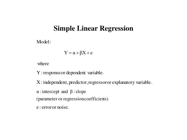
Simple Linear Regression. Data available : (X,Y). G oal : To predict the response Y. (i.e. to obtain the fitted response function f(X)). How to determine this regression function? (need to estimate the parameters.). Least Squares Fitting Method.

E N D
Data available:(X,Y) Goal:To predict the response Y. (i.e. to obtain the fitted response function f(X)) How to determine this regression function? (need to estimate the parameters.) Least Squares Fitting Method
Least Squares Regression Function: Least Squares Estimates
Terminology Fitted model True model Fitted regression function
REGRESSION ON MIDTERM GRADE Obs MIDTERM FINAL 1 68 75 2 49 63 3 60 57 4 68 88 5 97 88 6 82 79 7 59 82 8 50 73 9 73 90 10 39 62 11 71 70 12 95 96 13 61 76 14 72 75 15 87 85 16 40 40 17 66 74 18 58 70 19 58 75 20 77 72 Figure 1.4 SAS PROC PRINT output for the grade data problem.
TITLE ‘REGRESSION ON MIDTERM GRADE’; DATA; INPUT MIDTERM FINAL; CARDS; 68 75 49 63 60 57 . . 77 72 ; PROC PLOT; PLOT FINAL*MIDTERM=’O’ PRED*MIDTERM=’P’ / OVERLAY; LABEL FINAL=’FINAL’; PROC RANK NORMAL=VW; VAR RESID; RANKS NSCORE; • PROC PLOT; • PLOT RESID*NSCORE=’R’; • LABEL NSCORE=’NORMAL SCORE’; • RUN; PROC PRINT; PROC REG; MODEL FINAL=MIDTERM / P; OUTPUT PREDICTED=PRED RESIDUAL=RESID;
REGRESSION ON MIDTERM GRADE Model: MODEL1 Dependent Variable: FINAL Analysis of Variance Sum of Mean Source DF Squares Square F Value Pr > F Model 1 1774.44117 1774.44117 24.26 0.0001 Error 18 1316.55883 73.14216 Corrected Total 19 3091.00000 Root MSE 8.55232 R-Square 0.5741 Dependent Mean 74.50000 Adj R-Sq 0.5504 Coeff Var 11.47962 Parameter Estimates Parameter Standard Variable DF Estimate Error t Value Pr > |t| Intercept 1 34.56757 8.32984 4.15 0.0006 MIDTERM 1 0.60049 0.12192 4.93 0.0001
Dep Var Predicted Obs FINAL Value Residual 1 75.0000 75.4007 -0.4007 2 63.0000 63.9915 -0.9915 3 57.0000 70.5968 -13.5968 4 88.0000 75.4007 12.5993 5 88.0000 92.8149 -4.8149 6 79.0000 83.8076 -4.8076 7 82.0000 69.9963 12.0037 8 73.0000 64.5920 8.4080 9 90.0000 78.4032 11.5968 10 62.0000 57.9866 4.0134 11 70.0000 77.2022 -7.2022 12 96.0000 91.6139 4.3861 13 76.0000 71.1973 4.8027 14 75.0000 77.8027 -2.8027 15 85.0000 86.8100 -1.8100 16 40.0000 58.5871 -18.5871 17 74.0000 74.1998 -0.1998 18 70.0000 69.3959 0.6041 19 75.0000 69.3959 5.6041 20 72.0000 80.8051 -8.8051 Sum of Residuals 0 Sum of Squared Residuals 1316.55883 Predicted Residual SS (PRESS) 1668.47241
| 100 + | o | | o p p | o o | o | o p 80 + p o F | o p pp I | o o o o o N | o pp o o A | p p L | p | o o 60 + p | p o | | | | | 40 + o | -+------------+------------+------------+------------+------------+------------+------------+ 30 40 50 60 70 80 90 100 NOTE: 6 obs hidden. MIDTERM Figure 1.6 Output for the first PROC PLOT step for the grade data problem.
20 + | | | | R | R R 10 + | R R | e | R R R s | R i | d 0 +---------------------------------R---------R--R--------------------------------------------- u | R R a | R l | R R | R | R -10 + | | R | | | R -20 + | --+----------+----------+----------+----------+----------+----------+----------+----------+-- 55 60 65 70 75 80 85 90 95 Predicted Value of FINAL Figure 1.7 The remainder of the output from the first PROC PLOT step.
20 + | | | | R | R R 10 + | R R | e | R R R s | R i | d 0 + R R R u | R R a | R l | R R | R | R -10 + | | R | | | R -20 + | --+----------+----------+----------+----------+----------+----------+----------+----------+-- -2.0 -1.5 -1.0 -0.5 0.0 0.5 1.0 1.5 2.0 NORMAL SCORE
*Pearson’s Correlation Coefficient *Goal:The degree of linear correlation between two variables. The range lies between –1 and 1.
*Coefficient of Determination: the fraction of the variance in y that is explained by regression on x. Goal:may be used as an index of linearity for the relation of y to x. Definition:
120 + | o | | o | 100 + o | | o | o P | o R 80 + E | o o S | o S | o U | o R 60 + o o | o | o | o | o 40 + o o | o o | o o o | o | 20 + | ---+---------+---------+---------+---------+---------+---------+---------+---------+-- 10 15 20 25 30 35 40 45 50 VOLUME Figure 3.3: A plot of the air pressure data (an example of residual analysis).
| 30 + | | | | * | 20 + | R | e | * s |* i | d 10 + * * u | a | * l | * * | | * * 0 +------------------------------------------------------------------------------*------------- | * | * * | * * | * * | * * * * -10 + * * * | -+---------+---------+---------+---------+---------+---------+---------+---------+---------+- 16.357 25.007 33.658 42.308 50.959 59.609 68.259 76.910 85.560 94.210 Predicted Value of P Figure 3.4 The residual on fit plot after fitting the model P= a + b V + e to the air pressure data.
0.50 + | * | | * | 0.25 + | | * * * * * * | * * * R | * * * e 0.00 +-----------------------*--------------------------*------------------------ s | * i | * * * d | u | * a -0.25 + * l | * | * | | -0.50 + | | | * | -0.75 + ---+-------------+-------------+-------------+-------------+-------------+-- 20 40 60 80 100 120 Predicted Value of P Figure 3.5 The residual on the fit plot using the model P = a + b/V +e for the air pressure data.
Weighted Regression Problem: (unequal variance) Model: Claim:minimize Ordinary Regression Model: Claim:minimize
How to determine the weights? So the optimal weights are inversely proportional to the variances of the y.
PROC REG; MODEL P=VI; WIGHT W; OUTPUT P=FIT R=RES; DATA; SET; WRES=SQRT(W)*RES; DATA; INPUT V P; VI=1/V; CARDS; 48 29.1 . . . 12 117.6 ; PROC RANK NORMAL=VW; VAR WRES; RANKS NSCORE; PROC PLOT; PLOT WRES*FIT=’*’ / VREF=0 VPOS=30; POLT WRES*NSCORE=’*’ /VPOS=30; LABEL WRES=’WEIGHTED RESIDUAL’ NSCORE=’NORMAL SCORE’; RUN; PROC REG; MODEL P=VI; OUTPUT P=LSFIT; DATA; SET; W=1/LSFIT;
| 0.050 + | | * W | * E | I 0.025 + * * * G | * * * H | * T | * * * E | * * D 0.000 +-----------------------*--------------------------------------------------- | * R | * * * E | * S | I -0.025 + * D | * U | A | * L | -0.050 + * | | | | * -0.075 + | ---+-------------+-------------+-------------+-------------+-------------+-- 20 40 60 80 100 120 Predicted Value of P Figure 3.13 Weighted residual plot for a weighted fit of the model P = a + b/V + e to the air pressure data .
0.0002 + | | | * | * 0.0001 + * * | * | R | * * * e | * * s 0 +------*--------*-------------------------------*---------------*--------------------* i | * * * * d | * u | * * a | * l -0.0001 + * | | | | -0.0002 + | | | * | -0.0003 + | ---+---------------+---------------+---------------+---------------+---------------+-- -0.034 -0.029 -0.024 -0.019 -0.014 -0.009 Predicted Value of PT Figure 3.17 Residual on fit plot for the model –1/ P =α+ BV + e in air pressure data.
| | 0.0002 + | | | * | * 0.0001 + * * | * | R | * * * e | * * s 0 + * * * * * i | * * * * d | * u | * * a | * l -0.0001 + * | | | | -0.0002 + | | | * | -0.0003 + | ---+------------------+------------------+------------------+------------------+-- -2 -1 0 1 2 NORMAL SCORE Figure 3.18 Residual normal probability plot for the model –1/ P =α+ BV + e in air pressure data..
| | 0.0001 + * | * | * | | * 0.00005 + * * | * | * R | * e | * * s 0 +----------------------------------------------------*------------------------ i | * * * d | * * u | a | * * l -0.00005 + * | * * | | | * -0.0001 + | | | * | -0.00015 + | ---+-------+-------+-------+-------+-------+-------+-------+-------+-------+-- -0.033 -0.030 -0.027 -0.024 -0.021 -0.018 -0.016 -0.013 -0.010 -0.007 Predicted Value of PT Figure 3.19 Residual on fit plot for the model –1/ P =α+ BV + e in Example 3.4 after deleting the first data point.
| | 0.0001 + * | * | * | | * 0.00005 + * * | * | * R | * e | * * s 0 + * i | * * * d | * * u | a | * * l -0.00005 + * | * * | | | * -0.0001 + | | | * | -0.00015 + | ---+------------------+------------------+------------------+------------------+-- -2 -1 0 1 2 NORMAL SCORE Figure 3.20 Residual normal probability plot for the model –1/ P =α+ BV + e in Example 3.4 after deleting the first data point.
How to determine the weights of transformation T such that (assuming T is monotonic increasing)