Simple Linear Regression
Simple Linear Regression. (Session 02). Learning Objectives. At the end of this session, you will be able to understand the meaning of a simple linear regression model, its aims and terminology

Simple Linear Regression
E N D
Presentation Transcript
Simple Linear Regression (Session 02)
Learning Objectives At the end of this session, you will be able to • understand the meaning of a simple linear regression model, its aims and terminology • determine the best fitting line describing the relationship between a quantitative response (y) and a quantitative explanatory variable (x) • Interpret the unknown parameters of the regression line
An illustrative example Data on the next slide shows the average number of cigarettes smoked per adult in 1930 and the death rate per million in 1952 for sixteen countries. The question of interest is whether there is a relationship between the death rate (y) and level of smoking (x). Here both y and x are quantitative measurements.
Start by plotting - shows pattern -a straight line relationship seems plausible here.
Recall reasons for modelling • To determine which of (often) several factors explain variability in the key response of interest; • To summarise the relationship(s); • For predictive purposes, e.g. predicting y for given x’s, or identifying x’s that optimise y in some way; Note: Presence of an association between variables does not necessarily imply causation.
Describing the Regression Model Describe variation in response (here death rate) in terms of its relationship with the explanatory variable (here cig. numbers). Model : data = pattern + residual • can describe pattern as: a + bx , if straight line relationship seems reasonable • residual is unexplained variation - assumed to be random.
Simple Linear Regression Model If there is only one explanatory variable, we have a Simple Linear Regression Model. Here data = pattern + residual becomes: y = + x + where + x =pattern and = residual. • is called the intercept • is called the slope • the ’s represent the departure of the true line from the observed values.
Parameters of Model & Assumptions • and are the unknown parameters in the model. They are estimated from the data • The random error, , is assumed to have a • normal distribution • with constant variance (whatever the value of x) We shall return to these assumptions later.
Results of model fitting ------------------------------------------------------ deathrate|Coef. Std.Err. t P>|t| [95% Conf.Int.] ---------+-------------------------------------------- Cigars | .2410 .0544 4.43 0.001 .1245 .3577 Const. | 28.31 46.92 0.60 0.556 -72.34 128.95 ------------------------------------------------------ These are estimates of coefficients of the regression equation since this is a sample of data - precision quantified by standard errors Estimated equation is: y = 28.31 + 0.241 * x Note: The t and P>|t| columns will be discussed in the next session.
Interpreting model parameters • Slope (regression coefficient): If cigarettes smoked increases by 1 unit per year, death rate will increase by 0.24 units. In other words, if cigarettes smoked increases by 100 units, death rate will increase by 24 units. • Intercept of 28.31 only has meaning if the range of x values (cigarettes smoked) under study includes the value of zero. Here zero cigarettes smoked still gives an estimated death rate of 28.3
Predictions from the line The model equation can also be used to predict y at a given value of x Thus from y = 28.31 + 0.241 x, predicted death rate ( ) in a country where number of cigarettes smoked is x=1000, is given by = 28.31 + 0.241 (1000) = 269.3 Note: Predictions will be discussed in greater detail in Session 9.
Computation of model estimates (for reference only) Note: Can also write
Practical work follows to ensure learning objectives are achieved…

