Recent progress in EVLA-specific algorithms
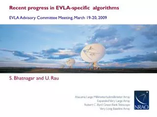
Recent progress in EVLA-specific algorithms. EVLA Advisory Committee Meeting, March 19-20, 2009. S. Bhatnagar and U. Rau. Imaging issues. Full beam, full bandwidth, full Stokes noise limited imaging Algorithmic R&D Requirements: PB corrections:

Recent progress in EVLA-specific algorithms
E N D
Presentation Transcript
Recent progress in EVLA-specific algorithms EVLA Advisory Committee Meeting, March 19-20, 2009 S. Bhatnagar and U. Rau
Imaging issues Full beam, full bandwidth, full Stokes noise limited imaging Algorithmic R&D Requirements: PB corrections: Rotation, Freq. & Poln. dependence, W-term (L-band) Multi-frequency Synthesis at 2:1 BWR PB scaling with frequency, Spectral Index variations Scale and frequency sensitive deconvolution Direction dependent corrections Time varying PB, pointing offsets, polarization
Calibration issues Band pass calibration Solution per freq. Channel (limited by SNR) Polynomial/spline solutions (also ALMA req.) Multiple Spectral Windows Direction dependent instrumental calibration Time varying PB, pointing offsets, ionospheric (L-band)/atmospheric (all bands) Polarization calibration Freq. Dependant leakage Beam polarization correction RFI flagging/removal Strong: Auto-, Semi-auto flagging Weak: Research problem
Imaging limits: Due to PB Limits due to asymmetric PB In-beam max. error @ 10% point: ~10000:1 Errors due to sources in the first side-lobe: 3x-5x higher Less of a problem for non-mosaicking observation at higher frequencies (>C-band) But similar problems for mosaicking at higher frequencies Limits due to antenna pointing errors In-beam and first side-lobe errors: ~10000:1 Similar limits for mosaicking at higher frequencies
Imaging limits: Due to PB Time varying PB gain Sources of time variability • PB rotationally asymmetric • PB rotation with PA • PB scaling with frequency • Antenna pointing errors Cross hand power pattern
Imaging limits: Due to bandwidth Frequency dependence Instrumental: PB scales by 2X is strongest error term Sky: Varying across the band – needs to be solved for during imaging (MFS) Limits due to sky spectral index variations: A source with Sp. Index ~1 can limit the imaging dynamic range to ~103-4
Wide-band static PB 10% 50% 90% Wide-band power pattern (3 Channels spanning 1 GHz of bandwidth) Gain change at first side lobe due to rotation Avg. PB Spectral Index (1-2GHz) Gain change in the main-lobe due to rotation
Algorithmic dependencies Wide-band, “narrow field” imaging Dominant error: Sky spectral index variation Post deconvolution PB corrections: Assume static PB Wide-band, wide-field imaging Dominant error: PB scaling Require time varying PB correction during deconvolution Pointing error correction Wide-band, full-beam, full-pol. Imaging Dominant error: PB scaling and PB polarization High DR imaging / mosaicking (ALMA) Requires all the above + Scale- and freq- sensitive modeling (multi-scale methods)
Progress (follow-up from last year) Wide field imaging W-Projection algorithm:[Published/in use] 3-10X faster (Cornwell, Golap, Bhatnagar, IEEE, 2008) Better handles complex fields Easier to integrated with other algorithms PB corrections Basic algorithm: AW-Projection algorithm: [Bhatnagar et al. A&A/ Testing] All-Stokes PB correction [Initial investigations] PB freq. Scaling [In progress] PB-measurements[In progress] Pointing SelfCal: [Sci. Testing] [Bhatnagar et al., EVLA Memo 84] Wide-band imaging [Basic algorithm Sci. Testing] U. Rau’s thesis: [in prep]
Correction for pointing errors and PB rotation: Narrow band Before correction After correction (Bhatnagar et al., EVLA Memo 100 (2006), A&A (2008)
Pointing SelfCal • Model image: 59 sources from NVSS. • Flux range ~2-200 mJy/beam (Bhatnagar et al., EVLA Memo 84) • Typical antenna pointing offsets for VLA as a function of time • Over-plotted data: Solutions at longer integration time • Noise per baseline as expected from EVLA
L-band imaging: Stokes-I & -V Stokes-I Stokes-V (10x improvement)
Wide-band imaging: Rau’s thesis Narrow field (EVLA Memo 101; Rau) Traditional MFS/bandwidth synthesis/Chan. Averaging inadequate for EVLA 2:1 BWR Post deconvolution PB correction Hybrid approach: DR ~104:1(Rau et al.,EVLA Memo 101) And requires more computing! MS-MFS (REF: in prep) MS-MFS + PB-correction Combining MS-MFS with AW-Projection Initial integration + testing in progress (with real data)
Extending MFS: Basics algorithm Image at reference frequency Average Spectral Index Gradient in Spectral Index True Images MS-MFS (new) Traditional-MFS (Rau, Corwnell) (EVLA Memo 101)
Application to M87: Fresh results Stokes-I Sp. Ndx. (No PB correction) (Rau, Owen) Sp. Ndx. variation
Wideband PB correction Before PB correction PB=50% After PB correction 3C286 Stokes-I (Rau, Bhatnagar)
Computing challenges Significant increase in computing for wide-band and wide-field imaging Larger convolution kernels MFS and MS-MFS loads: Equivalent of Ntaylor * Nscales imaging load. Typical Ntaylor = 3, Nscales = 5 Direction dependent terms Corrections and calibration as expensive as imaging I/O load Near future data volume: 100-200 GB / 8hr by mid-2010 20-50 passes through the data (flagging + calibration + imaging)
CASA Terabyte Initiative Develop pipelines for end-to-end processing Primary calibration, flagging, Imaging, SelfCal Test Cluster parameters (Paid for by ALMA & EVLA) 16 nodes Each node: 8GB RAM, 200GB disk, 8 cores Total cost: ~$70K Current effort: Data volume: 100 GB Integration time=1s; Total length: 2hr No. of channels: 1024 across 32 Sub-bands Future tests with 500 GB and 1 TB data sizes
Computing & I/O load: Single node Data: 100 GB, 512 Channels, 4K x 4K x 512 Stokes-I imaging 4 CPU, 16 GB RAM computer I/O : Compute = 3:2 Conclusions: Simple processing is I/O dominated Image deconvolution is the most expensive step Most expensive part of imaging is the Major Cycle Exploit data parallelism as the first goal Total effective I/O ~1 TB (iterations)
Parallelization: Initial results Spectral line imaging: (8GB RAM per node) Strong scaling with number of nodes & cube size Dominated by data I/O and handling of image cubes in the memory 1024 x 1024 x 1024 imaging 1-Node run-time : 50hr 16-node run : 1.5 hr Continuum imaging: (No PB-correction or MFS) Requires inter-node I/o Dominated by data i/o 1024 x 1024 imaging: 1-node run-time : 9hr 16-node run-time : 70min (can be reduced upto 50%)
Plan: Parallelization & Algorithms • Initial goal for parallelization • Pipelines to exploit data parallelization • Get cluster h/w requirements • Collaboration with UVa • New developments: Algorithms research • Imaging • Integration of various DD terms (W-term, PB-corrections, Sp.Ndx....) • Wide(er) field • Full polarization • Better scale-sensitive (multi-scale) deconvolution • Calibration • DD calibration • New developments: Computing • OpenMP to exploit multi-CPU/core computers • Robust pipelines for e2e processing
Computing challenges (backup slide) Residual computation (Major Cycle) Most expensive part of post processing I/O limited Required in iterative calibration and imaging Component modeling (Minor cycle) Required in MS and MS-MFS Computation limited Direction dependent calibration As expensive as imaging