QUESTIONS
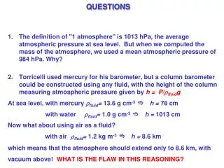
QUESTIONS. The definition of "1 atmosphere" is 1013 hPa , the average atmospheric pressure at sea level. But when we computed the mass of the atmosphere, we used a mean atmospheric pressure of 984 hPa . Why?

QUESTIONS
E N D
Presentation Transcript
QUESTIONS • The definition of "1 atmosphere" is 1013 hPa, the average atmospheric pressure at sea level. But when we computed the mass of the atmosphere, we used a mean atmospheric pressure of 984 hPa. Why? • Torricelli used mercury for his barometer, but a column barometercould be constructed using any fluid, with the height of the columnmeasuring atmospheric pressure given by h = P/rfluidg At sea level, with mercury rfluid= 13.6 g cm-3 e h = 76 cm with water rfluid= 1.0 g cm-3 e h = 1013 cm Now what about using air as a fluid? with airrfluid= 1.2 kg m-3 e h = 8.6 km which means that the atmosphere should extend only to 8.6 km, with vacuum above! WHAT IS THE FLAW IN THIS REASONING?
CHAPTER 3: SIMPLE MODELS The atmospheric evolution of a species X is given by the continuity equation deposition emission transport (flux divergence; U is wind vector) local change in concentration with time chemical production and loss (depends on concentrations of other species) This equation cannot be solved exactly e need to construct model (simplified representation of complex system) Improve model, characterize its error Design observational system to test model Design model; make assumptions needed to simplify equations and make them solvable Evaluate model with observations Define problem of interest Apply model: make hypotheses, predictions
TYPES OF SOURCES Natural Surface: terrestrial and marine highly variable in space and time, influenced by season, T, pH, nutrients… eg. oceanic sources estimated by measuring local supersaturation in water and using a model for gas-exchange across interface =f(T, wind velocity….) Natural In situ: eg. lightning (NOx) N2 NOx, volcanoes (SO2, aerosols) generally smaller than surface sources on global scale but important b/c material is injected into middle/upper troposphere where lifetimes are longer Anthropogenic Surface: eg. mobile, industry, fires good inventories for combustion products (CO, NOx, SO2) for US and EU Anthropogenic In situ: eg. aircraft, tall stacks Secondary sources: tropospheric photochemistry Injection from the stratosphere: transport of products of UV dissociation (NOx, O3) transported into troposphere (strongest at midlatitudes, important source of NOx in the UT)
TYPES OF SINKS • Wet Deposition: falling hydrometeors (rain, snow, sleet) carry trace species to the surface • in-cloud nucleation (depending on solubility) • scavenging (depends on size, chemical composition) • Soluble and reactive trace gases are more readily removed • Generally assume that depletion is proportional to the conc (1st order loss) • Dry Deposition: gravitational settling; turbulent transport • particles > 20 µm gravity (sedimentation) • particles < 1 µm diffusion • rates depend on reactivity of gas, turbulent transport, stomatal resistance and together define a deposition velocity (vd) • In situ removal: • chain-terminating rxn: OH●+HO2● H2O + O2 • change of phase: SO2 SO42- (gas dissolved salt) Typical values vd: Particles:0.1-1 cm/s Gases: vary with srf and chemical nature (eg. 1 cm/s for SO2)
RESISTANCE MODEL FOR DRY DEPOSITION Deposition Flux: Fd = -vdC Vd = deposition velocity (m/s) C = concentration Use a resistance analogy, where rT=vd-1 C3 For gases at steady state can relate overall flux to the concentration differences and resistances across the layers: 0 0 Aerodynamic resistance = ra C2 Quasi-laminar layer resistance = rb C1 Canopy resistance = rc C0=0 For particles, assume that canopy resistance is zero (so now C1=0), and need to include particle settling (settling velocity=vs) which operates in parallel with existing resistances. End result: Reference: Seinfeld & Pandis, Chap 19
Atmospheric “box”; spatial distribution of X within box is not resolved ONE-BOX MODEL Chemical production Chemical loss Inflow Fin Outflow Fout X L P D E Flux units usually [mass/time/area] Deposition Emission (turnover time) Lifetimes add in parallel: (because fluxes add linearly) Loss rate constants add in series:
ASIDE: LIFETIME VS RADIOACTIVE HALF-LIFE Both express characteristic times of decay, what is the relationship? ½ life:
EXAMPLE: GLOBAL BOX MODEL FOR CO2reservoirs in PgC, flows in Pg C yr-1 atmospheric content (mid 80s) = 730 Pg C of CO2 annual exchange land = 120 Pg C yr-1 annual exchange ocean= 90 Pg C yr-1 (now ~816 PgCO2) Human Perturbation IPCC [2001]
SPECIAL CASE: SPECIES WITH CONSTANT SOURCE, 1st ORDER SINK Steady state solution (dm/dt = 0) Initial condition m(0) • Characteristic time t = 1/k for • reaching steady state • decay of initial condition If S, k are constant over t >> t, then dm/dt g0 and mg S/k: "steady state"
TWO-BOX MODELdefines spatial gradient between two domains F12 m2 m1 F21 Mass balance equations: (similar equation for dm2/dt) If mass exchange between boxes is first-order: e system of two coupled ODEs (or algebraic equations if system is assumed to be at steady state)
Illustrates long time scale for interhemispheric exchange; can use 2-box model to place constraints on sources/sinks in each hemisphere
TWO-BOX MODEL(with loss) mo = m1+m2 T Q m1 m2 S1 S2 Lifetimes: If at steady state sinks=sources, so can also write: Now if define: α=T/Q, then can say that: Maximum α is 1 (all material from reservoir 1 is transferred to reservoir 2), and therefore turnover time for combined reservoir is the sum of turnover times for individual reservoirs. For other values of α, the turnover time of the combined reservoir is reduced.
EULERIAN RESEARCH MODELS SOLVE MASS BALANCE EQUATION IN 3-D ASSEMBLAGE OF GRIDBOXES The mass balance equation is then the finite-difference approximation of the continuity equation. Solve continuity equation for individual gridboxes • Models can presently afford • ~ 106 gridboxes • In global models, this implies a horizontal resolution of 100-500 km in horizontal and ~ 1 km in vertical • Drawbacks: “numerical diffusion”, computational expense
EULERIAN MODEL EXAMPLE Summertime Surface Ozone Simulation Here the continuity equation is solved for each 2x2.5 grid box. They are inherently assumed to be well-mixed [Fiore et al., 2002]
IN EULERIAN APPROACH, DESCRIBING THE EVOLUTION OF A POLLUTION PLUME REQUIRES A LARGE NUMBER OF GRIDBOXES Fire plumes over southern California, 25 Oct. 2003 A Lagrangian “puff” model offers a much simpler alternative
PUFF MODEL: FOLLOW AIR PARCEL MOVING WITH WIND [X](x, t) In the moving puff, wind [X](xo, to) …no transport terms! (they’re implicit in the trajectory) Application to the chemical evolution of an isolated pollution plume: [X]b [X] In pollution plume,
COLUMN MODEL FOR TRANSPORT ACROSS URBAN AIRSHED Temperature inversion (defines “mixing depth”) Emission E In column moving across city, Solution: [X] x 0 L
LAGRANGIAN RESEARCH MODELS FOLLOW LARGE NUMBERS OF INDIVIDUAL “PUFFS” C(x, to+Dt) Individual puff trajectories over time Dt • ADVANTAGES OVER EULERIAN MODELS: • Computational performance (focus puffs on region of interest) • No numerical diffusion • DISADVANTAGES: • Can’t handle mixing between puffs a can’t handle nonlinear processes • Spatial coverage by puffs may be inadequate C(x, to) Concentration field at time t defined by n puffs
FLEXPART: A LAGRANGIAN MODEL Retroplume (20 days): Trinidad Head, Bermuda x Emissions Map (NOx) = Region of Influence But no chemistry, deposition, convection here [Cooper et al., 2005]