Download
1 / 9
90 likes | 246 Views
Raw satellite data from the GOME instrument (ESA). Earth Observation DEMO. 2 different jobs are executed on the TESTBED , using data provided via the sandbox model. Processing of raw GOME data to ozone profiles With OPERA (KNMI). LIDAR data. Validate GOME ozone profiles

E N D
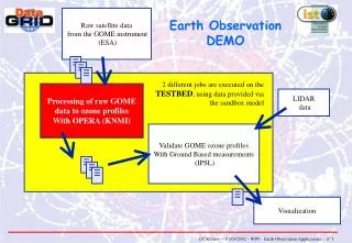
Raw satellite data from the GOME instrument (ESA) Earth Observation DEMO 2 different jobs are executed on the TESTBED, using data provided via the sandbox model Processing of raw GOME data to ozone profiles With OPERA (KNMI) LIDAR data Validate GOME ozone profiles With Ground Based measurements (IPSL) Visualization
DEMO background Earth Observation data are scattered over various institutes: ESA receives ‘raw’ data from their ERS satellite, and store their data across various archive centers in Europe. Other institutes use these data to generate ’higher’ products with in-house developed algorithms. These kind of data are used to give information about our climate system and can be used to steer weather models. To provide good quality data other data sources are used for validation, like comparison with ground based measurements.
Used DataGrid commands dg-job-submit run-opera.jdl > my_output_1 my_Job_Id=`grep "https://" my_output_1`while test $rep != "OutputReady" -a $rep != "Aborted" do sleep 4 dg-job-status $my_Job_Id > my_output_2 set rep=`grep Status my_output_2 | awk {print $3}` donedg-job-get-output $my_Job_Id > my_output_3rap=`grep "tmp" my_output_3`cp $rap/* /home/vegtevd/output/cd /home/vegtevd/output/tar xvf *.tarcd Lv2cat *.el2
OPERA application (KNMI) From wave spectra measured by the GOME instrument on the ERS satellite ozone profiles can be calculated. ESA provides these spectra as level 1 data. This level 1 data is then processed using OPERA to produce ozone profiles, a level 2 product. The algorithm and s/w (OPERA) are developed by KNMI. GOME takes ~30.000 usable measurements for ozone profile retrieval per day. The calculation of 1 profile takes ~2 min on a 800Mhz PIII. One day of profiles will take 40 days on 1 computer.
Raw satellite data from the GOME instrument (ESA) Earth Observation DEMO 2 different jobs are executed on the TESTBED, using data provided via the sandbox model Processing of raw GOME data to ozone profiles With OPERA (KNMI) LIDAR data Validate GOME ozone profiles with Ground Based measurements (IPSL) Visualization
Validation application (IPSL) Produced profiles by OPERA are validated by IPSL using ground based LIDAR measurements. Since the LIDAR data are in-situ, pre-selection of the global GOME data has to be performed to create a dataset which is geograpically and temporally in coincidence. The main function of the program is to perform statistical operations like the bias between GOME and LIDAR data for different altitudes and its standard deviations. The output of the validation program are 2 plots, generated by xmgr.
Used JDL file Executable = "o3gome-lidar_xmgr.final";StdOutput = "appli.out";StdError = "appli.err";InputSandbox = {"/home/leroy/DEMO_190202/o3gome-lidar_xmgr.final","/home/leroy/DEMO_190202/obs20001019.dat","/home/leroy/DEMO_190202/obs20001002.dat","/home/leroy/DEMO_190202/obs20001003.dat","/home/leroy/DEMO_190202/obs20001004.dat","/home/leroy/DEMO_190202/obs20001005.dat","/home/leroy/DEMO_190202/obs20001006.dat","/home/leroy/DEMO_190202/select_coinc.exe","/home/leroy/DEMO_190202/data_process_demoxmgr","/home/leroy/DEMO_190202/oho30010.gol"}; OutputSandbox = {"out_proc.dat","profil_gome.dat","profil_lidar.dat","appli.out","appli.err"};Requirements = other.OpSys == “RH 6.2”;RetryCount = 10;Rank = other.MaxCpuTime; The produced profiles by OPERA are validated by IPSL using ground based LIDAR measurements. One Month of data (gome and lidar data) is used to do a analysis between the different measurements The result is visualized using xmgr.
Validation output figure 1: Estimation of the bias between Gome and Lidar using one month of data. figure 2 : example of 2 profiles : Comparison between Gome profile and lidar profile for the 2nd October 2000.
Why Earth Observation needs DataGrid • Earth Observation data is large and scattered over the globe in different organizations. One year of raw ENVISAT data will be in the order of 400 Terabytes, Users of these data are located at different sites, which will use these data in various ways: production of operational products which have to be generated within strict time frames, or perform an analysis on a month of satellite data to see if degradation of the instrument is occurring. The grid will provide the Earth Observation community a collaborative environment. • Large computing resources are a must to perform analysis of satellite data One measurement of 1.5 sec will take 2 min to be processed for an ozone profile on 1 CPU. A typical validation period consists of 1 month of data, resulting in ~2 million CPU minutes, so this would take 3 years to process on 1 computer !, While desired response time must be in the order of hours/days. Using Datagrid will be the mechanism to tackle these issues.