Understanding Discrete Linear Inverse Problems: Methods and Applications in Estimation

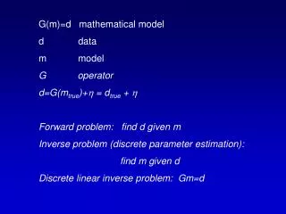
1. G(m)=d mathematical model d data m model G operator d=G(mtrue)+ = dtrue +  Forward problem: find d given m Inverse problem (discrete parameter estimation): find m given d Discrete linear inverse problem: Gm=d

2. G(m)=d mathematical model Discrete linear inverse problem: Gm=d Method of Least Squares: Minimize E=∑ ei2 = ∑ (diobs-dipre)2 dipre Diobs zi o ei o o o o

3. E=eTe=(d-Gm)T(d-Gm) =∑ [di-∑Gijmj] [di-∑Gikmk] =∑ ∑ mj mk ∑ Gij Gik -2∑ mj ∑ Gijdi + ∑ di di ∂/∂mq [∑ ∑ mj mk ∑ Gij Gik ] = ∑ ∑ [jqmk+mjkq]∑GijGik = 2 ∑ mk ∑ Giq Gik -2 ∂/∂mq [∑ mj ∑ Gijdi ] = -2∑jq∑Gijdi = -2∑ Giqdi ∂/∂mq [∑didi]=0 i j k j k ij i i j k ij k i k i j I j i i i

4. ∂/∂mq = 0 =2 ∑ mk ∑ Giq Gik - 2∑ Giqdi In matrix notation: GTGm - GTd = 0 mest = [GTG]-1GTd assuming [GTG]-1 exists This is the least squares solution to Gm=d k i i

5. Example of fitting a straight line mest = [GTG]-1GTd assuming [GTG]-1 exists m ∑ xi ∑ xi ∑ xi2 1 1 … 11 x1 [GTG]= 1 x2 = x1 x2 .. xm . 1 xm [GTG]-1 = m ∑ xi -1 ∑ xi ∑ xi2

6. Example of fitting a straight line mest = [GTG]-1GTd assuming [GTG]-1 exists ∑ di ∑ xi di 1 1 … 1 d1 [GTd]= d2 = x1 x2 .. xm . dm [GTG]-1 GTd= m ∑ xi -1 ∑ xi ∑ xi2 ∑ di ∑ xi di

7. The existence of the Least Squares Solution mest = [GTG]-1GTd assuming [GTG]-1 exists Consider the straight line problem with only 1 data point ? ? ? m ∑ xi -1 1 x1 -1 [GTG]-1 = = ∑ xi ∑ xi2 x1 x12 o The inverse of a matrix is proportional to the reciprocal of the determinant of the matrix, i.e., [GTG]-1 1/(x12-x12), which is clearly singular, and the formula for the least squares fails.

8. Classification of inverse problems: Over-determined Under-determined Mixed-determined Even-determined

9. Over-determined problems: Too much information contained in Gm=d to possess an exact solution … Least squares gives a ‘best’ approximate solution.

10. Even-determined problems: Exactly enough information to determine the model parameters. There is only one solution and it has zero prediction error

11. Under-determined Problems: Mixed-determined problems - non-zero prediction error Purely underdetermined problems - zero prediction error

12. Purely Under-determined Problems: # of parameters > # of equations Possible to find more than 1 solution with 0 prediction error (actually infinitely many) To obtain a solution, we must add some information not contained in Gm=d : a priori information Example: Fitting a straight line through a single data point, we may require that the line passes through the origin Common a priori assumption: Simple model solution best. Measure of simplicity could be Euclidian length, L=mTm = ∑ mi2

13. Purely Under-determined Problems: Problem: Find the mest that minimizes L=mTm = ∑ mi2 subject to the constraint that e=d-Gm=0 (m)= L+∑ i ei = ∑ mi2 +∑ i [ di - ∑ Gijmj ] ∂(m)/∂mq= 2 ∑ mi ∂mi/∂mq-∑ i ∑ Gij∂mj /∂mq] = 2mq - ∑ iGiq = 0 In matrix notation: 2m = GT (1), along with Gm=d (2) Inserting (1) into (2) we get d=Gm=G[GT/2] , = 2[GGT]-1d and inserting into (1): m = GT [GGT]-1d - solution exist when purely underdetermined

14. Mixed-determined problems Over Under Mixed determined determined determined Partition into overdetermined and underdetermined parts, solve by LS and minimum norm - SVD (later) Minimize some combination of the prediction error and solution length for the unpartitioned model (m)=E+2L=eTe+2mTm mest=[GTG+2I]-1GTd - damped least squares

15. Mixed-determined problems • (m)=E+2L=eTe+2mTm • mest=[GTG+2I]-1GTd - damped least squares • Regularization parameter 0th-order Tikhonov Regularization ||m||  ||Gm-d|| Min ||m||2, ||Gm-d||2< min ||Gm-d||2, ||m||2 <  ||m||  ‘L-curves’ ||Gm-d||

16. Other A Priori Info: Weighted Least Squares Data weighting (weighted measures if prediction error) E=eTWee We is a weighting matrix, defining relative contribution of each individual error to the total prediction error (usually diagonal). For example, for 5 observations, the 3rd may be twice as accurately determined as the others: Diag(We)=[1, 1, 2, 1, 1]T Completely overdetermined problem: mest=[GTWeG]-1GTWed

17. Other A Priori Info: Constrained Regression di=m1+m2xi Constraint: line must pass through (x’,d’): d’=m1+m2x’ Fm= [1 x’] [m1 m2]T = [d’] Similar to the unconstrained solution (2.5) we get: m1est M ∑ xi 1 -1 ∑ di m2est = ∑ xi ∑xi2 x’ ∑ xidi 11 x’ 0 d’ o o (x’,d’) o o d x o Unconstrained solution: [GTG]-1 GTd= M ∑ xi -1 ∑ xi ∑ xi2 ∑ di ∑ xi di

18. Other A Priori Info: Weighting model parameters Instead of using minimum length as solution simplicity, One may impose smoothness in the model: -1 1 m1 -1 1 m2 l = . . . = Dm . . . -1 1 mN D is the flatness matrix L=lTl=[Dm]T[Dm]=mTDTDm=mTWmm, Wm=DTD firsth-order Tikhonov Regularization - min||Gm-d||22+||Lm||22

19. Other A Priori Info: Weighting model parameters Instead of using minimum length as solution simplicity, One may impose smoothness in the model: 1 -2 1 m1 1 -2 1 m2 l = . . . . = Dm . . . . 1 -2 1 mN D is the roughness matrix L=lTl=[Dm]T[Dm]=mTDTDm=mTWmm, Wm=DTD 2nd-order Tikhonov Regularization- min||Gm-d||22+||Lm||22