Download
1 / 21
360 likes | 954 Views
Design of Line, Circle & Ellipse Algorithms. Slope-Intercept Formula For A Line Given a third point on the line: P = (x,y) Slope = (y - y 1 )/(x - x 1 ) = (y 2 - y 1 )/(x 2 - x 1 ) Solving For y y = [(y 2 -y 1 )/(x 2 -x 1 )]x + [-(y 2 -y 1 )/(x 2 -x 1 )]x 1 + y 1

E N D
Slope-Intercept Formula For A Line Given a third point on the line: P = (x,y) Slope = (y - y1)/(x - x1) = (y2 - y1)/(x2 - x1) Solving For y y = [(y2-y1)/(x2-x1)]x + [-(y2-y1)/(x2-x1)]x1 + y1 therefore y = Mx + B where M = [(y2-y1)/(x2-x1)] B = [-(y2-y1)/(x2-x1)]y1 + y1 Basic Math Review Cartesian Coordinate System 6 P = (x,y) 5 4 P2 = (x2,y2) 3 2 1 P1 = (x1,y1) 1 3 4 5 6 7 RISE y2-y1 SLOPE = = RUN x2-x1
Length of line segment between P1 and P2: L = sqrt[ (x2-x1)2 + (y2-y1)2 ] Midpoint of a line segment between P1 and P3: P2 = ( (x1+x3)/2 , (y1+y3)/2 ) Two lines are perpendicular iff 1) M1 = -1/M2 or 2) Cosine of the angle between them is 0. Other Helpful Formulas
Given points P1 = (x1, y1) and P2 = (x2, y2) x = x1 + t(x2-x1) y = y1 + t(y2-y1) t is called the parameter. When t = 0 we get (x1,y1) t = 1 we get (x2,y2) As 0 < t < 1 we get all the other points on the line segment between (x1,y1) and (x2,y2). Parametric Form Of The Equation OfA 2D Line Segment
1. Must compute integer coordinates of pixels which lie on or near a line or circle. 2. Pixel level algorithms are invoked hundreds or thousands of times when an image is created or modified. 3. Lines must create visually satisfactory images. Lines should appear straight Lines should terminate accurately Lines should have constant density Line density should be independent of line length and angle. 4. Line algorithm should always be defined. Basic Line and Circle Algorithms
Procedure DDA(X1,Y1,X2,Y2 :Integer); Var Length, I :Integer; X,Y,Xinc,Yinc :Real; Begin Length := ABS(X2 - X1); If ABS(Y2 - Y1) > Length Then Length := ABS(Y2-Y1); Xinc := (X2 - X1)/Length; Yinc := (Y2 - Y1)/Length; X := X1; Y := Y1; DDA (digital differential analyzer) creates good lines but it is too time consuming due to the round function and long operations on real values. Simple DDA Line Algorithm{Based on the parametric equation of a line} For I := 0 To Length Do Begin Plot(Round(X), Round(Y)); X := X + Xinc; Y := Y + Yinc End {For} End; {DDA}
Compute which pixels should be turned on to represent the line from (6,9) to (11,12). Length := Max of (ABS(11-6), ABS(12-9)) = 5 Xinc := 1 Yinc := 0.6 Values computed are: (6,9), (7,9.6), (8,10.2), (9,10.8), (10,11.4), (11,12) DDA Example
Since the equation for a circle on radius r centered at (0,0) is x2 + y2 = r2, an obvious choice is to plot y = ±sqrt(r2 - x2) for -r <= x <= r. This works, but is inefficient because of the multiplications and square root operations. It also creates large gaps in the circle for values of x close to R (and clumping for x near 0). A better approach, which is still inefficient but avoids the gaps is to plot x = r cosø y = r sinø as ø takes on values between 0 and 360 degrees. Simple Circle Algorithms
Assumptions: Assume we wish to draw a line between points (0,0) and (a,b) with slope M between 0 and 1 (i.e. line lies in first octant). The general formula for a line is y = Mx + B where M is the slope of the line and B is the y-intercept. From our assumptions M = b/a and B = 0. Therefore y = (b/a)x + 0 is f(x,y) = bx – ay = 0 (an equation for the line). If (x1,y1) lie on the line with M = b/a and B = 0, then f(x1,y1) = 0. Fast Lines Using The Midpoint Method (a,b) (0,0)
For lines in the first octant, the next pixel is to the right or to the right and up. Assume: Distance between pixels centers = 1 Having turned on pixel P at (xi, yi), the next pixel is T at (xi+1, yi+1) or S at (xi+1, yi). Choose the pixel closer to the line f(x, y) = bx - ay = 0. The midpoint between pixels S and T is (xi + 1,yi + 1/2). Let e be the difference between the midpoint and where the line actually crosses between S and T. If e is positivethe line crosses above the midpoint and is closer to T. If e is negative, the line crosses below the midpoint and is closer to S. To pick the correct point we only need to know the sign of e. T = (xi + 1, yi + 1) (xi +1, yi + 1/2 + e) e (xi +1,yi + 1/2) P = (xi,yi ) S = (xi + 1, yi ) Fast Lines (cont.)
f(xi+1,yi+ 1/2 + e) = b(xi+1) - a(yi+ 1/2 + e) = b(xi + 1) - a(yi + 1/2) -ae = f(xi + 1, yi + 1/2) - ae = 0 Let di = f(xi + 1, yi + 1/2) = ae; di is known as the decision variable. Since a >= 0, di has the same sign as e. Algorithm: If di >= 0 Then Choose T = (xi + 1, yi + 1) as next point di+1 = f(xi+1 + 1, yi+1 + 1/2) = f(xi +1+1,yi +1+1/2) = b(xi +1+1) - a(yi +1+1/2) = f(xi + 1, yi + 1/2) + b - a = di + b - a Else Choose S = (xi + 1, yi) as next point di+1 = f(xi+1 + 1, yi+1 + 1/2) = f(xi +1+1,yi +1/2) = b(xi +1+1) - a(yi +1/2) = f(xi + 1, yi + 1/2) + b = di + b Fast Lines - The Decision Variable
Fast Line Algorithm x := 0; y := 0; d := b - a/2; For i := 0 to a do Plot(x,y); If d >= 0 Then x := x + 1; y := y + 1; d := d + b – a Else x := x + 1; d := d + b End End The initial value for the decision variable, d0, may be calculated directly from the formula at point (0,0). d0 = f(0 + 1, 0 + 1/2) = b(1) - a(1/2) = b - a/2 Therefore, the algorithm for a line from (0,0) to (a,b) in the first octant is: Note: The only non-integer value is a/2. If we then multiply by 2 to get d' = 2d, we can do all integer arithmetic using only the operations +, -, and left-shift. The algorithm still works since we only care about the sign, not the value of d.
We can also generalize the algorithm to work for lines beginning at points other than (0,0) by giving x and y the proper initial values. This results in Bresenham's Line Algorithm. Bresenham’s Line Algorithm Begin {Bresenham for lines with slope between 0 and 1} a := ABS(xend - xstart); b := ABS(yend - ystart); d := 2*b - a; Incr1 := 2*(b-a); Incr2 := 2*b; If xstart > xend Then x := xend; y := yend Else x := xstart; y := ystart End For I := 0 to a Do Plot(x,y); x := x + 1; If d >= 0 Then y := y + 1; d := d + incr1 Else d := d + incr2 End End {For Loop} End {Bresenham} Note: This algorithm only works for lines with Slopes between 0 and 1
We only need to calculate the values on the border of the circle in the first octant. The other values may be determined by symmetry. Assume a circle of radius r with center at (0,0). Procedure Circle_Points(x,y :Integer); Begin Plot(x,y); Plot(y,x); Plot(y,-x); Plot(x,-y); Plot(-x,-y); Plot(-y,-x); Plot(-y,x); Plot(-x,y) End; Circle Drawing Algorithm
Consider only the first octant of a circle of radius r centered on the origin. We begin by plotting point (r,0) and end when x < y. The decision at each step is whether to choose the pixel directly above the current pixel or the pixel which is above and to the left. Assume Pi = (xi, yi) is the current pixel. Ti = (xi, yi +1) is the pixel directly above Si = (xi -1, yi +1) is the pixel above and to the left. Fast Circles
f(x,y) = x2 + y2 - r2 = 0 f(xi - 1/2 + e, yi + 1) = (xi - 1/2 + e)2 + (yi + 1)2 - r2 = (xi- 1/2)2 + (yi+1)2 - r2 + 2(xi-1/2)e + e2 = f(xi - 1/2, yi + 1) + 2(xi - 1/2)e + e2 = 0 Let di = f(xi - 1/2, yi+1) = -2(xi - 1/2)e - e2 Thus, If e < 0 then di > 0 so choose point S = (xi - 1, yi + 1). di+1 = f(xi - 1 - 1/2, yi + 1 + 1) = ((xi - 1/2) - 1)2 + ((yi + 1) + 1)2 - r2 = di - 2(xi -1) + 2(yi + 1) + 1 = di + 2(yi+1- xi+1) + 1 If e >= 0 then di <= 0 so choose point T = (xi, yi + 1). di+1 = f(xi - 1/2, yi + 1 + 1) = di + 2yi+1 + 1 Fast Circles - The Decision Variable (xi -1/2, yi + 1) T = (xi ,yi +1) e S = (xi -1,yi +1) P = (xi ,yi )
The initial value of di is d0 = f(r - 1/2, 0 + 1) = (r - 1/2)2 + 12 - r2 = 5/4 - r {1-r can be used if r is an integer} When point S = (xi - 1, yi + 1) is chosen then di+1 = di + -2xi+1 + 2yi+1 + 1 When point T = ( xi , yi + 1) is chosen then di+1 = di + 2yi+1 + 1 Fast Circles - Decision Variable (cont.)
Begin {Circle} x := r; y := 0; d := 1 - r; Repeat Circle_Points(x,y); y := y + 1; If d <= 0 Then d := d + 2*y + 1 Else x := x - 1; d := d + 2*(y-x) + 1 End Until x < y End; {Circle} Fast Circle Algorithm Procedure Circle_Points(x,y :Integer); Begin Plot(x,y); Plot(y,x); Plot(y,-x); Plot(x,-y); Plot(-x,-y); Plot(-y,-x); Plot(-y,x); Plot(-x,y) End;
The circle algorithm can be generalized to work for an ellipse but only four way symmetry can be used. F(x,y) = b2x2 + a2y2 -a2b2 = 0 (0,b) (x, y) (-x, y) (a,0) (-a,0) (x, -y) (-x, -y) (0,-b) Fast Ellipses
The circle algorithm can be generalized to work for an ellipse but only four way symmetry can be used. F(x,y) = b2x2 + a2y2 -a2b2 = 0 All the points in one quadrant must be computed. Since Bresenham's algorithm is restricted to only one octant, the computation must occur in two stages. The changeover occurs when the point on the ellipse is reached where the tangent line has a slope of ±1. In the first quadrant, this is where the line y = x intersects the ellipses. Fast Ellipses (0,b) y = x (x, y) (-x, y) (a,0) (-a,0) (x, -y) (-x, -y) (0,-b)
Bresenham, J.E., "Ambiguities In Incremental Line Rastering," IEEE Computer Graphics And Applications, Vol. 7, No. 5, May 1987. Eckland, Eric, "Improved Techniques For Optimising Iterative Decision- Variable Algorithms, Drawing Anti-Aliased Lines Quickly And Creating Easy To Use Color Charts," CSC 462 Project Report, Department of Computer Science, North Carolina State University (Spring 1987). Foley, J.D. and A. Van Dam, Fundamentals of Interactive Computer Graphics, Addison-Wesley 1982. Newman, W.M and R.F. Sproull, Principles Of Interactive Computer Graphics, McGraw-Hill, 1979. Van Aken J. and Mark Novak, "Curve Drawing Algorithms For Raster Display," ACM Transactions On Graphics, Vol. 4, No. 3, April 1985. Line and Circle References