Download
1 / 63
630 likes | 1.5k Views
Acknowledgements. Bength

E N D
2. Bength & Linda Muth�n
Mplus: http://www.statmodel.com/
Alan A. Acock
Department of HDFS
Oregon State University
Brigitte Wanner
GRIP
University of Montr�al Before I being I would like to acknowledge that a lot the material you will see over the next two days is based on great material I have encountered from three primary sources
First via the makers of Mplus . . . I have attended two workshops and I HIGHLY recommend it.
Second is material from Alan Acock and Brigitte Wanner (a colleague from the GRIP) whom some of you may know. Before I being I would like to acknowledge that a lot the material you will see over the next two days is based on great material I have encountered from three primary sources
First via the makers of Mplus . . . I have attended two workshops and I HIGHLY recommend it.
Second is material from Alan Acock and Brigitte Wanner (a colleague from the GRIP) whom some of you may know.
3. Introduction to Mplus
Mplus & prog. language
Preparing data
Descriptive statistics
Basic growth Curve Model
Basic Model and Assumption
Mplus code
Interpreting Output & Graphs
Quadratic terms
Mplus program
Interpreting Output & Graphs Missing values in growth models
Introduction
Mplus code
Output
Multiple group models
At the same time
As categorical predictors to show differences in intercept and/or slope
Additional models
There are many . . .
4. When you launch Mplus, this is the screen you first see. This is the input window and you write your code in this window. I will show you the different elements of Mplus programming language soon. But we have to start at the beginning.
There is also an output window. But you do not see this automatically. You have to run the code in your input window first. Once Mplus has finished processing your code, it replaces the input window with the output window When you launch Mplus, this is the screen you first see. This is the input window and you write your code in this window. I will show you the different elements of Mplus programming language soon. But we have to start at the beginning.
There is also an output window. But you do not see this automatically. You have to run the code in your input window first. Once Mplus has finished processing your code, it replaces the input window with the output window
5. Here is an example of the input and output windows.
The input window is in the back � notice the color coding. This is an active window. The output window Here is an example of the input and output windows.
The input window is in the back � notice the color coding. This is an active window. The output window
6. Different commands divided into a series of sections
TITLE
DATA (required)
VARIABLE (required)
DEFINE
ANALYSIS
MODEL
OUTPUT
SAVEDATA
MONTECARLO Here is an example of the input and output windows.
The input window is in the back � notice the color coding. This is an active window. The output window Here is an example of the input and output windows.
The input window is in the back � notice the color coding. This is an active window. The output window
7. TITLE:
Everything after �Title:� is the title and the title ends when �Data:� appears
DATA:
Tells Mplus where to find the file containing the data.
�E:\Growth_Curves\ClassData.dat�
Without a specific path, Mplus will look in the same folder where the Mplus code is saved Here is an example of the input and output windows.
The input window is in the back � notice the color coding. This is an active window. The output window Here is an example of the input and output windows.
The input window is in the back � notice the color coding. This is an active window. The output window
8. VARIABLE:
Series of subcommands that tell Mplus . . .
Names are names of variables (8 characters max; case sensitive in certain versions)
Missing are all (-99) ; tells Mplus user defined missing values
Use variables are names variables to use in the analysis. Useful if have larger data file for multiple purposes/analysis. IMPORTANT
ANALYSIS:
Tells Mplus what type of analysis and estimator will be used
Type = basic ; (default)
We start with basic, but as we progress though , you will see that the analysis TYPE will change We start with basic, but as we progress though , you will see that the analysis TYPE will change
9. MODEL:
This contains the basic model statements
Y ON X ; ! regression
F1 BY var1@1 var2 var3 var4 ; ! Latent factors
var1 WITH var2 ; !correlation
OUTPUT:
Lists specific statistical and graphical output wanted
Will get to this in the next section
We start with basic, but as we progress though , you will see that the analysis TYPE will change We start with basic, but as we progress though , you will see that the analysis TYPE will change
10. This is a fictitious dataset of 2278 youth between the ages of 12 to 17.
We have non-violent delinquency scores between the ages 12 to 17, and violent delinquency only through 12 to 15
About 50% male, 66% from families with mothers and fathers; 13% receive meal vouchers for school; 66% white.
So. Lets talk about elements of the SPSS code. GET gets the data; RECODE puts our missing at -99; this is important for Mplus as we will discuss when we come to missing data, etc.;
WRITE OUTFILE ID has to be character variable with no decimals. Mplus does not like IDs with decimals. And then we are putting the rest of the variables (14) to columns that are 8 characters wide, and with 2 decimal points
The WRITE OUTFILE will place the file in the folder you tell it to. In this example, Drive E>Subfolder GROWTHCURVES> file name GCWS.DAT
This is a fictitious dataset of 2278 youth between the ages of 12 to 17.
We have non-violent delinquency scores between the ages 12 to 17, and violent delinquency only through 12 to 15
About 50% male, 66% from families with mothers and fathers; 13% receive meal vouchers for school; 66% white.
So. Lets talk about elements of the SPSS code. GET gets the data; RECODE puts our missing at -99; this is important for Mplus as we will discuss when we come to missing data, etc.;
WRITE OUTFILE ID has to be character variable with no decimals. Mplus does not like IDs with decimals. And then we are putting the rest of the variables (14) to columns that are 8 characters wide, and with 2 decimal points
The WRITE OUTFILE will place the file in the folder you tell it to. In this example, Drive E>Subfolder GROWTHCURVES> file name GCWS.DAT
11. Here is an example of a basic analysis. From this basic analysis, you will receive basic descriptives, i.e, the output contains means, SEs, correlations and variance-covariance matrices.
So, let�s walk through the sections of Mplus code.
TITLE;
DATA;
VARIABLE (notice the idvariable=; and something else new is the CATEGORICAL are (Default is continuous in MPLUS)
ANALYSIS;Here is an example of a basic analysis. From this basic analysis, you will receive basic descriptives, i.e, the output contains means, SEs, correlations and variance-covariance matrices.
So, let�s walk through the sections of Mplus code.
TITLE;
DATA;
VARIABLE (notice the idvariable=; and something else new is the CATEGORICAL are (Default is continuous in MPLUS)
ANALYSIS;
12. Create Mplus data file from SPSS
Write the translation file in SPSS
Check to make sure your data is correctly created
Conduct basic Mplus analysis
Write the Mplus code
We start with basic, but as we progress though , you will see that the analysis TYPE will change We start with basic, but as we progress though , you will see that the analysis TYPE will change
13. Introduction to Mplus
Mplus & prog. language
Preparing data
Descriptive statistics
Basic growth Curve Model
Basic Model and Assumption
Mplus code
Interpreting Output & Graphs
Quadratic terms
Mplus program
Interpreting Output & Graphs Missing values in growth models
Introduction
Mplus code
Output
Multiple group models
At the same time
As categorical predictors to show differences in intercept and/or slope
Additional models
There are many . . .
14. General latent variable framework
Implemented in Mplus program Muth�n and Muth�n (1998-2007)
Latent Growth Curve modeling / Structural Equation Modeling (SEM) is linked to Random Coefficient Growth Modeling / Multilevel modeling
Latent Growth Curve modeling (single population) is a �case� of Growth Mixture Modeling (we cover this tomorrow)
Here is an example of the input and output windows.
The input window is in the back � notice the color coding. This is an active window. The output window Here is an example of the input and output windows.
The input window is in the back � notice the color coding. This is an active window. The output window
15. Average growth within a population and its variation
Continuous latent variables (growth factors) capture individual differences in development
Intercept (mean starting value)
Slope (rate of growth)
Quadratic term (leveling off, or coming down)
16. observed variables
continuous
censored
binary
ordinal
count
combinations
continuous latent variables
measurement models (show an example later today)
Outcomes � or the behavior you will examine in growth curves, can be either observed or continous latent variables.
For observed, you can model just about any type of variable in Mplus, from continious, cenosred (restricted in range), binary, ordinal, counts, and even combinations of these variables.
For latent variables, you can model growth curves on top of measurement models.
We are focusing on observed variables, but towards the end of today, I will give you an example of growth curves on measurement models.Outcomes � or the behavior you will examine in growth curves, can be either observed or continous latent variables.
For observed, you can model just about any type of variable in Mplus, from continious, cenosred (restricted in range), binary, ordinal, counts, and even combinations of these variables.
For latent variables, you can model growth curves on top of measurement models.
We are focusing on observed variables, but towards the end of today, I will give you an example of growth curves on measurement models.
17. Estimating a basic growth curve using Mplus is quite easy.
In general, start simple, move to more complex Starting easy should include data screening to evaluate the distributions of the variables, patterns of missing values, and possible outliers. We will start with fitting a basic growth curve. Even if you have a theoretically specified model that is complex, always start with the simplest model and gradually add the complexity. Here we will show how structural equation modeling conceptualizes a latent growth curves, show the Mplus program, explain the new program features, and interpret the output.
Before showing a figure to represent a growth curve, we will examine a small sample of our observations:
So, right from the beginning, based on 25 of the youth, we can see considerable variation. I will point out a few individuals. Starting easy should include data screening to evaluate the distributions of the variables, patterns of missing values, and possible outliers. We will start with fitting a basic growth curve. Even if you have a theoretically specified model that is complex, always start with the simplest model and gradually add the complexity. Here we will show how structural equation modeling conceptualizes a latent growth curves, show the Mplus program, explain the new program features, and interpret the output.
Before showing a figure to represent a growth curve, we will examine a small sample of our observations:
So, right from the beginning, based on 25 of the youth, we can see considerable variation. I will point out a few individuals.
18. This figure is much simpler than it first appears.
The key variables are the two latent variables labeled the Intercept and the Slope.
The intercept represents the initial level and is sometimes called the initial level for this reason. It is the estimated initial level and its value may differ from the actual mean for D12 because in this case we have a linear growth model. It may differ from the mean of D12 by a lot when covariates are added because of the adjustments for the covariates.
Unless the covariates are centered, it usually makes sense to just call it an intercept rather than the initial level. The intercept is identified by the constant loadings of 1.0 going to each delinquency score. Some programs call the intercept the constant, representing the constant effect.
The slope is identified by fixing the values of the paths to each delinquency variable. In a publication you normally would not show the path to delinquency age 12, since this is fixed at 0.0.
We fix the other paths at 1.0, 2,0, 3.0, 4.0, and 5.0 Where did we get these values? The first year is the base year or year zero (with the effect of locating the intercept at the initial measurement). Delinquency was measured each subsequent year so these are scored 1.0 through 5.0. Other values are possible. Suppose the survey was not done at ages 15 and 16, so that we had 4 time points rather than 6. We would use paths of 0.0, 1.0, 2.0, 3.0, and 6.0 for years 12, 13, 14 and 17.
It is also possible to fix the first couple years and then allow the subsequent waves to be free. This might make sense for a developmental process where the yearly intervals may not reflect the developmental rate. Developmental time may be quite different than chronological time (language acquisition in years 1,2 and 3). This has the effect of �stretching� or �shrinking� time to the pattern of the data (Curran & Hussong, 2003). An advantage of this approach is that it uses fewer degrees of freedom than adding a quadratic slope.
The individuals in our sample will each have their own
delinquency score for each year
Intercept and
Slope represent the overall trend.
Features to notice in the figure:
The individual variation around the Intercept and Slope are represented in by the arrows pointing to the Intercept and Slope. These are the variance in the intercept and slope around their respective means.
We expect there would be substantial variance in both of these as some individuals have a higher or lower starting delinquency and some individuals will increase (or decrease) their delinquency at a different rate than the average growth rate.
In addition to the mean intercept and slope, each individual will have their own intercept and slope. We say the intercept and the slope are random effects.
They are random in the sense that each individual may have a steeper or flatter slope than the mean slope and
Each individual may have a higher or lower initial level than the mean intercept.
In our sample of 25 individuals shown in the previous slide, notice one adolescent starts with high delinquency around 12 whereas most start with low levels of delinqency. Some have a delinquency that increases immediately and peaks around 13, whereas others peak around 15.
The variances, are critical if we are going to explore more complex models with covariates (e.g., gender, poverty) that might explain why some individuals have a steeper or less steep growth rate than the average.
The arrows pointing at the observed delinquency scores indicate individual error terms for each year. Some years may move above or below the growth trend described by our Intercept and Slope. Sometimes it might be important to allow error terms to be correlated, especially subsequent pairs such as ages 12-13;13-14;14-15, etc.This figure is much simpler than it first appears.
The key variables are the two latent variables labeled the Intercept and the Slope.
The intercept represents the initial level and is sometimes called the initial level for this reason. It is the estimated initial level and its value may differ from the actual mean for D12 because in this case we have a linear growth model. It may differ from the mean of D12 by a lot when covariates are added because of the adjustments for the covariates.
Unless the covariates are centered, it usually makes sense to just call it an intercept rather than the initial level. The intercept is identified by the constant loadings of 1.0 going to each delinquency score. Some programs call the intercept the constant, representing the constant effect.
The slope is identified by fixing the values of the paths to each delinquency variable. In a publication you normally would not show the path to delinquency age 12, since this is fixed at 0.0.
We fix the other paths at 1.0, 2,0, 3.0, 4.0, and 5.0 Where did we get these values? The first year is the base year or year zero (with the effect of locating the intercept at the initial measurement). Delinquency was measured each subsequent year so these are scored 1.0 through 5.0. Other values are possible. Suppose the survey was not done at ages 15 and 16, so that we had 4 time points rather than 6. We would use paths of 0.0, 1.0, 2.0, 3.0, and 6.0 for years 12, 13, 14 and 17.
It is also possible to fix the first couple years and then allow the subsequent waves to be free. This might make sense for a developmental process where the yearly intervals may not reflect the developmental rate. Developmental time may be quite different than chronological time (language acquisition in years 1,2 and 3). This has the effect of �stretching� or �shrinking� time to the pattern of the data (Curran & Hussong, 2003). An advantage of this approach is that it uses fewer degrees of freedom than adding a quadratic slope.
The individuals in our sample will each have their own
delinquency score for each year
Intercept and
Slope represent the overall trend.
Features to notice in the figure:
The individual variation around the Intercept and Slope are represented in by the arrows pointing to the Intercept and Slope. These are the variance in the intercept and slope around their respective means.
We expect there would be substantial variance in both of these as some individuals have a higher or lower starting delinquency and some individuals will increase (or decrease) their delinquency at a different rate than the average growth rate.
In addition to the mean intercept and slope, each individual will have their own intercept and slope. We say the intercept and the slope are random effects.
They are random in the sense that each individual may have a steeper or flatter slope than the mean slope and
Each individual may have a higher or lower initial level than the mean intercept.
In our sample of 25 individuals shown in the previous slide, notice one adolescent starts with high delinquency around 12 whereas most start with low levels of delinqency. Some have a delinquency that increases immediately and peaks around 13, whereas others peak around 15.
The variances, are critical if we are going to explore more complex models with covariates (e.g., gender, poverty) that might explain why some individuals have a steeper or less steep growth rate than the average.
The arrows pointing at the observed delinquency scores indicate individual error terms for each year. Some years may move above or below the growth trend described by our Intercept and Slope. Sometimes it might be important to allow error terms to be correlated, especially subsequent pairs such as ages 12-13;13-14;14-15, etc.
19. What is new in this program?
The first change is that we modify the Usevariables are: subcommand to only include the delinquncy variables since we are doing a growth curve for these variables.
We drop the Analysis: section because we are doing basic growth curve and can use the default options.
We have added a Model: Mplus has a simple built in way of restricting the paramters to fit the assumptions our model. There is a single line to describe our model:
i s | delinq1@0 delinq2@1 delinq3@2 delinq4@3 delinq5@4 delinq6@5 ;
In this line the �I� and �s� stand for intercept and slope. We could have called these anything such as intercept and slope or initial and trend. The vertical line, | , tells Mplus that it is about to define an intercept and slope.
There are defaults that we do not need to note. For example,
the intercept is defined by a constant of 1.0 for each delinquency variable. This is normally the case, so it is a default. The slope is defined by fixing the path from the slope to delinquency at age 12 at 0, the slope of age 13 at 1, etc. The @ sign is used for �at.� Don�t forget the semi-colon to end the command.
Mplus assumes there is random error, ei for each variable and that these are uncorrelated.
Mplus also assumes that there is a residual variance for both the intercept and slope (RI and RS) and that these covary. Therefore, we do not need to mention this.
The last additional section in our Mplus program is for selecting what output we want Mplus to provide. There are many optional outputs of the program and we will only illustrate a few of these. The Output: section has the following lines
The first line, Sampstat Mod(3.84) asks for sample statistics and modification indices for parameters we might free, as long as doing so would reduce chi-square by 3.84 (corresponding to the .05 level). We do not bother with parameter estimates that would have less effect than this.
Next comes the Plot: subcommand, and we say that we want Type is Plot3; for our output. This gives us the descriptive statistics and graphs for the growth curve.
The last line of the program specifies the series to plot. By entering the variables with an (*) at the end we are setting a path at 0.0 for bmi97, 1.0 for bmi98, etc.What is new in this program?
The first change is that we modify the Usevariables are: subcommand to only include the delinquncy variables since we are doing a growth curve for these variables.
We drop the Analysis: section because we are doing basic growth curve and can use the default options.
We have added a Model: Mplus has a simple built in way of restricting the paramters to fit the assumptions our model. There is a single line to describe our model:
i s | delinq1@0 delinq2@1 delinq3@2 delinq4@3 delinq5@4 delinq6@5 ;
In this line the �I� and �s� stand for intercept and slope. We could have called these anything such as intercept and slope or initial and trend. The vertical line, | , tells Mplus that it is about to define an intercept and slope.
There are defaults that we do not need to note. For example,
the intercept is defined by a constant of 1.0 for each delinquency variable. This is normally the case, so it is a default. The slope is defined by fixing the path from the slope to delinquency at age 12 at 0, the slope of age 13 at 1, etc. The @ sign is used for �at.� Don�t forget the semi-colon to end the command.
Mplus assumes there is random error, ei for each variable and that these are uncorrelated.
Mplus also assumes that there is a residual variance for both the intercept and slope (RI and RS) and that these covary. Therefore, we do not need to mention this.
The last additional section in our Mplus program is for selecting what output we want Mplus to provide. There are many optional outputs of the program and we will only illustrate a few of these. The Output: section has the following lines
The first line, Sampstat Mod(3.84) asks for sample statistics and modification indices for parameters we might free, as long as doing so would reduce chi-square by 3.84 (corresponding to the .05 level). We do not bother with parameter estimates that would have less effect than this.
Next comes the Plot: subcommand, and we say that we want Type is Plot3; for our output. This gives us the descriptive statistics and graphs for the growth curve.
The last line of the program specifies the series to plot. By entering the variables with an (*) at the end we are setting a path at 0.0 for bmi97, 1.0 for bmi98, etc.
20. Number of observations 1554 ! listwise, an alternative is FIML estimation
Number of dependent variables 7 !these are the delinwquency scores
Number of continuous latent variables 2 !these are the intercept and slope Number of observations 1554 ! listwise, an alternative is FIML estimation
Number of dependent variables 7 !these are the delinwquency scores
Number of continuous latent variables 2 !these are the intercept and slope
21. These have the standard interpretations.
It is okay if the fit is not perfect here because when we add the covariates we may get a better fit. We can also, for example, examine from modification outputs if correlating errors for consecutive time points in delinquency increases goodness of fit.
The chi-square is significant as it usually is for a large sample because any model is not likely to be a perfect fit for data. However, the CFI = .63 and TLI = .656 are both in the very bad range (i.e., over .96 is very good). The RMSEA is .226 and this is not very good. Ideally, this should be below .06, and a value that is not below .08 is considered problematic.
The Standardized RMSR = .177 is not acceptable (less than .05)
In SUMMARY � BAD MODEL FIT!!!sThese have the standard interpretations.
It is okay if the fit is not perfect here because when we add the covariates we may get a better fit. We can also, for example, examine from modification outputs if correlating errors for consecutive time points in delinquency increases goodness of fit.
The chi-square is significant as it usually is for a large sample because any model is not likely to be a perfect fit for data. However, the CFI = .63 and TLI = .656 are both in the very bad range (i.e., over .96 is very good). The RMSEA is .226 and this is not very good. Ideally, this should be below .06, and a value that is not below .08 is considered problematic.
The Standardized RMSR = .177 is not acceptable (less than .05)
In SUMMARY � BAD MODEL FIT!!!s
22. ! the I and S are all fixed so no tests for them.
! The slope and intercept are correlated, the covariance is
! -.719, z = -7.527, p < .001 (WITH means covariance in Mplus)
!Initial level, intercept = 2.146, (Delinquency starts at 2.146) z = 23.868; p < .001
!Slope = .668 (delinquency goes down -0.062each year), z = -2.982; P < .05
Delinquency goes down?? Does this seem right? Anyone have an idea of what is going on here??
In the basic analysis we saw delinquency peaked.! the I and S are all fixed so no tests for them.
! The slope and intercept are correlated, the covariance is
! -.719, z = -7.527, p < .001 (WITH means covariance in Mplus)
!Initial level, intercept = 2.146, (Delinquency starts at 2.146) z = 23.868; p < .001
!Slope = .668 (delinquency goes down -0.062each year), z = -2.982; P < .05
Delinquency goes down?? Does this seem right? Anyone have an idea of what is going on here??
In the basic analysis we saw delinquency peaked.
23. ! Variances, Ri and Rs in the figure, are both significant. This is what covariates will try to explain�why do some youth start higher/lower and have a different trend, i.e., slope, for the delinquency?
! Following are the residual variances for the observed variables, hence they are the errors, ei�s in our figure.! Variances, Ri and Rs in the figure, are both significant. This is what covariates will try to explain�why do some youth start higher/lower and have a different trend, i.e., slope, for the delinquency?
! Following are the residual variances for the observed variables, hence they are the errors, ei�s in our figure.
24. ! Many of these changes make no sense. We could let the path of the slope to delinq2 (or age 12) be free and chi-square would drop by about 52 points.
! These �with� statements are for correlated errors. Some make sense, some don�t.
It is important to use modification indices as a guidline and only those that make sense
There is also variation in how reviewers will react, even to correlation residuals in adjacent times for delinquency
Last �
! We do not pay much attention to these intercepts because Mplus automatically fixes them at zero. Before freeing these, it would make more sense to free some of the coefficients for slopes, e.g., 0, 1, *, *, *, * or to try a quadratic slope as will be shown in the next section! Many of these changes make no sense. We could let the path of the slope to delinq2 (or age 12) be free and chi-square would drop by about 52 points.
! These �with� statements are for correlated errors. Some make sense, some don�t.
It is important to use modification indices as a guidline and only those that make sense
There is also variation in how reviewers will react, even to correlation residuals in adjacent times for delinquency
Last �
! We do not pay much attention to these intercepts because Mplus automatically fixes them at zero. Before freeing these, it would make more sense to free some of the coefficients for slopes, e.g., 0, 1, *, *, *, * or to try a quadratic slope as will be shown in the next section
25. Here are Some of the Available Plots
It is often useful to show the actual means for a small random sample of participants. These are Sample Means.
Click on Graphs
Observed Individual Values
This gives you a menu where you can make some selectionsHere are Some of the Available Plots
It is often useful to show the actual means for a small random sample of participants. These are Sample Means.
Click on Graphs
Observed Individual Values
This gives you a menu where you can make some selections
26. Next, lets look at a plot of the actual means and the estimated means using our linear growth model. Click on
Graphs and then select
Sample and estimated means.Next, lets look at a plot of the actual means and the estimated means using our linear growth model. Click on
Graphs and then select
Sample and estimated means.
27. Run basic growth curve model in Mplus
Write Mplus code
Go through results and annotate the meaning of different parts of the results
Examine 2 graphs
Individual observed values
Sample estimated means based on model
Next, lets look at a plot of the actual means and the estimated means using our linear growth model. Click on
Graphs and then select
Sample and estimated means.Next, lets look at a plot of the actual means and the estimated means using our linear growth model. Click on
Graphs and then select
Sample and estimated means.
28. Introduction to Mplus
Mplus & prog. language
Preparing data
Descriptive statistics
Basic growth Curve Model
Basic Model and Assumption
Mplus code
Interpreting Output & Graphs
Quadratic terms
Mplus program
Interpreting Output & Graphs Missing values in growth models
Introduction
Mplus code
Output
Multiple group models
At the same time
As categorical predictors to show differences in intercept and/or slope
Additional models
There are many . . .
29. This graph is useful to seeing if there is a nonlinear trend. It is simple to add a quadratic term, if the curve is departing from linearity. The previous graph clearly showed that a slope is not sufficient to characterize the growth of delinquency. In addition, the relative fit indices were not within acceptable ranges, and the mean trend based on the model indicated a peaking distribution. A quadratic might pick this up by having a curve that peaks and drops in mid adolesence.
We now add a third latent variable so we will have the Intercept, Slope, and the new latent variable called the Quadratic trend. Like the first two, the Quadratic trend will have a residual variance (RQ) that will freely covariate with the residual variance of the intercept and slope. The paths from the quadratic trend to the individual BMI variables will be the square of the path from the Linear trend to the delinquency variables. Hence the values for the linear trend will remain 0.0, 1.0, 2.0, 3.0, 4.0, and 5.0. For the quadratic these values will be 0.0, 1.0, 4.0, 9.0, 16.0, and 25.0.This graph is useful to seeing if there is a nonlinear trend. It is simple to add a quadratic term, if the curve is departing from linearity. The previous graph clearly showed that a slope is not sufficient to characterize the growth of delinquency. In addition, the relative fit indices were not within acceptable ranges, and the mean trend based on the model indicated a peaking distribution. A quadratic might pick this up by having a curve that peaks and drops in mid adolesence.
We now add a third latent variable so we will have the Intercept, Slope, and the new latent variable called the Quadratic trend. Like the first two, the Quadratic trend will have a residual variance (RQ) that will freely covariate with the residual variance of the intercept and slope. The paths from the quadratic trend to the individual BMI variables will be the square of the path from the Linear trend to the delinquency variables. Hence the values for the linear trend will remain 0.0, 1.0, 2.0, 3.0, 4.0, and 5.0. For the quadratic these values will be 0.0, 1.0, 4.0, 9.0, 16.0, and 25.0.
30. All we have to do is add a �q� to the model statement
Mplus will know that the quadratic, q (we could use any name) will have values that are the square of the values for the slope, s.All we have to do is add a �q� to the model statement
Mplus will know that the quadratic, q (we could use any name) will have values that are the square of the values for the slope, s.
31. ! We have lost 4 degrees of freedom
mean for the quadratic slope,
variance for the quadratic slope,
covariance of the Rq with Ri
covariance with Rq with Rs
! The fit is MUCH better
Again, the chi-square is significant as it usually is for a large sample because any model is not likely to be a perfect fit for data. Chisquare, however, has drastically decreased (1283 to 102).
This time, the CFI = .97 and TLI = .97 are both very good (i.e., over .96 is very good). The RMSEA is .07 and this better but not excellent. Ideally, this should be below .06, and a value that is not below .08 is considered problematic.
The Standardized RMSR = .041 is acceptable (less than .05)
! We have lost 4 degrees of freedom
mean for the quadratic slope,
variance for the quadratic slope,
covariance of the Rq with Ri
covariance with Rq with Rs
! The fit is MUCH better
Again, the chi-square is significant as it usually is for a large sample because any model is not likely to be a perfect fit for data. Chisquare, however, has drastically decreased (1283 to 102).
This time, the CFI = .97 and TLI = .97 are both very good (i.e., over .96 is very good). The RMSEA is .07 and this better but not excellent. Ideally, this should be below .06, and a value that is not below .08 is considered problematic.
The Standardized RMSR = .041 is acceptable (less than .05)
32. ! Results for I and S are same as above. The paths for Q are simply the squared values
! The Negative slope, -.064, for quadratic suggests a leveling off and decrease in the growth curve.! Results for I and S are same as above. The paths for Q are simply the squared values
! The Negative slope, -.064, for quadratic suggests a leveling off and decrease in the growth curve.
33. The fit is so better because the estimated means and observed means are so close.
However, as shown, there is still significance variance among individual adolescents that needs to be explained.
The fit is so better because the estimated means and observed means are so close.
However, as shown, there is still significance variance among individual adolescents that needs to be explained.
34. Same routine, but here we are going to look at estimated curves per 20 individuals.
Notice that each of these is a curve, but they start at different initial levels and have different trajectories. So, it seems there is almost normative bump along adolescence. However, there may be a trend of high decreasing levels and increasing over time.
We may want to use covariates to explain these differences in the initial levels and growth trajectories. This will be addressed in future the last section today. Same routine, but here we are going to look at estimated curves per 20 individuals.
Notice that each of these is a curve, but they start at different initial levels and have different trajectories. So, it seems there is almost normative bump along adolescence. However, there may be a trend of high decreasing levels and increasing over time.
We may want to use covariates to explain these differences in the initial levels and growth trajectories. This will be addressed in future the last section today.
35. Run growth curve model with quradratic term
Write Mplus code
Go through results and annotate the meaning of different parts of the results
Examine 2 graphs
Estimated means based on model
Sample individual values
36. Introduction to Mplus
Mplus & prog. language
Preparing data
Descriptive statistics
Basic growth Curve Model
Basic Model and Assumption
Mplus code
Interpreting Output & Graphs
Quadratic terms
Mplus program
Interpreting Output & Graphs Missing values in growth models
Introduction
Mplus code
Output
Multiple group models
At the same time
As categorical predictors to show differences in intercept and/or slope
Additional models
There are many . . .
37. Mplus has two ways of working with missing values
full information maximum likelihood estimation with missing values (FIML)
Multiple imputations.
Imputing multiple datasets
Estimating the model for each of these datasets
Then pooling the estimates and standard errors
Mplus has two ways of working with missing values. The simplest is to use full information maximum likelihood estimation with missing values (FIML). This uses all available data. For example, some adolescents were interviewed all six years but others may have skipped one, two, or even more years. We use all available information with this approach.
The second approach is to utilize multiple imputations. Multiple imputation involves imputing multiple datasets (usually 5-10) using appropriate procedures, Estimating the model for each of these datasets, and Then pooling the estimates and standard errors.
When the standard errors are pooled this way, they incorporate the variability across the 5-10 solutions and are thereby produced unbiased estimates of standard errors. Multiple imputations can be done with:
Norm, a freeware program that works for normally distributed, continuous variables and is often used even on dichotomized variables.
A Stata user has written a program called ICE that is an implementation of the S-Plus program called MICE, that has advantages over Norm. It does the imputation by using different estimation models for outcome variables that are continuous, counts, or categorical. See Royston (2005).
SAS PROC MI
Mplus can read these multiple datasets, estimate the model for each dataset, and pool the estimates and their standard errors. Mplus has two ways of working with missing values. The simplest is to use full information maximum likelihood estimation with missing values (FIML). This uses all available data. For example, some adolescents were interviewed all six years but others may have skipped one, two, or even more years. We use all available information with this approach.
The second approach is to utilize multiple imputations. Multiple imputation involves imputing multiple datasets (usually 5-10) using appropriate procedures, Estimating the model for each of these datasets, and Then pooling the estimates and standard errors.
When the standard errors are pooled this way, they incorporate the variability across the 5-10 solutions and are thereby produced unbiased estimates of standard errors. Multiple imputations can be done with:
Norm, a freeware program that works for normally distributed, continuous variables and is often used even on dichotomized variables.
A Stata user has written a program called ICE that is an implementation of the S-Plus program called MICE, that has advantages over Norm. It does the imputation by using different estimation models for outcome variables that are continuous, counts, or categorical. See Royston (2005).
SAS PROC MI
Mplus can read these multiple datasets, estimate the model for each dataset, and pool the estimates and their standard errors.
38. We will not illustrate the multiple imputation approach because that involves working with other programs to impute the datasets. However, the Mplus User�s Guide, discusses how you specify the datasets in the Data: section. We will illustrate the FIML approach because it is widely used and easily implemented�and doesn�t require explaining another software package.
The conceptual model does not change with missing values. The programming for implementing the FIML solution changes very little. You will recall that we did not need an Analysis: section in our program for doing a growth curve. However, we do need one when we are doing a growth curve with missing values and using FIML estimation. Directly above the Model command we insert
Analysis:
Type = General Missing H1 ;
Estimator = MLR ;
Type = General Missing H1; this line is the key change.
The missing tells Mplus to do the full information maximum likelihood estimation.
The H1 is necessary to get sample statistics in our output.
In the Output: section, we also add a single word, patterns. This will give us a lot of information about patterns of missing values. We will see just what patterns there are, the frequency of occurrence of each pattern, and the percentage of data present for each covariance estimate.We will not illustrate the multiple imputation approach because that involves working with other programs to impute the datasets. However, the Mplus User�s Guide, discusses how you specify the datasets in the Data: section. We will illustrate the FIML approach because it is widely used and easily implemented�and doesn�t require explaining another software package.
The conceptual model does not change with missing values. The programming for implementing the FIML solution changes very little. You will recall that we did not need an Analysis: section in our program for doing a growth curve. However, we do need one when we are doing a growth curve with missing values and using FIML estimation. Directly above the Model command we insert
Analysis:
Type = General Missing H1 ;
Estimator = MLR ;
Type = General Missing H1; this line is the key change.
The missing tells Mplus to do the full information maximum likelihood estimation.
The H1 is necessary to get sample statistics in our output.
In the Output: section, we also add a single word, patterns. This will give us a lot of information about patterns of missing values. We will see just what patterns there are, the frequency of occurrence of each pattern, and the percentage of data present for each covariance estimate.
39. Number of cases with missing on all variables: 2
Notice, we are two youth short of the total sample now (2,278)
2276 ! We had 1544 observations using listwise deletion.
It is important to say, prior to this stage, we would have examined if the patterns of missing were meaningful. I will give a handout with references for this topic. Number of cases with missing on all variables: 2
Notice, we are two youth short of the total sample now (2,278)
2276 ! We had 1544 observations using listwise deletion.
It is important to say, prior to this stage, we would have examined if the patterns of missing were meaningful. I will give a handout with references for this topic.
40. An �x� mean the data are present. Pattern 1 -- no missing values Look at frequencies (1544 � listwise deletion)
! Pattern 2 � missing Delinq6 (210)
! We might want to set some minimum standard and drop observations that do not meet that. For example, we might drop people who are missing their delinquency for more than 3 waves. Or at least test results for such a model versus a model in which youth with at least 1 data point are allowed into the analysisAn �x� mean the data are present. Pattern 1 -- no missing values Look at frequencies (1544 � listwise deletion)
! Pattern 2 � missing Delinq6 (210)
! We might want to set some minimum standard and drop observations that do not meet that. For example, we might drop people who are missing their delinquency for more than 3 waves. Or at least test results for such a model versus a model in which youth with at least 1 data point are allowed into the analysis
41. ! We have 72.8% of the 2276 observations answering both delinquent1 and delinquent6! We have 72.8% of the 2276 observations answering both delinquent1 and delinquent6
42. ! Notice that although the trends are in the same direciton, the means are a bit higher compared to the the results of the �basic� analysis that had the 1544 observations using listwise deletion. This may be due to 1,200 person difference between the analysis. It may be wise to select individuals with at least 3 data point and then compare these individiuals to the listwise deleted (1544). Most like would be less severe differences.
! The chi-square is about twice as large when we use FIML estimation with missing values, in part because the sample is so much bigger. Still there are some fit problems Both the CFI and TLI are a bit low to be ideal (under .96). In addition, th RMSEA is a bit high, and that is the most widely used measure of fit.! Notice that although the trends are in the same direciton, the means are a bit higher compared to the the results of the �basic� analysis that had the 1544 observations using listwise deletion. This may be due to 1,200 person difference between the analysis. It may be wise to select individuals with at least 3 data point and then compare these individiuals to the listwise deleted (1544). Most like would be less severe differences.
! The chi-square is about twice as large when we use FIML estimation with missing values, in part because the sample is so much bigger. Still there are some fit problems Both the CFI and TLI are a bit low to be ideal (under .96). In addition, th RMSEA is a bit high, and that is the most widely used measure of fit.
43. Run growth curve model with missing analysis
Write Mplus code
Go through results and annotate how the results change when using missing data analysis
44. Introduction to Mplus
Mplus & prog. language
Preparing data
Descriptive statistics
Basic growth Curve Model
Basic Model and Assumption
Mplus code
Interpreting Output & Graphs
Quadratic terms
Mplus program
Interpreting Output & Graphs Missing values in growth models
Introduction
Mplus code
Output
Multiple group models
At the same time
As categorical predictors to show differences in intercept and/or slope
Additional models
There are many . . .
45. Gender
Boys higher in delinquency
Several ways
Compare models
Step 1: fit multiple model group and allow estimated parameters to vary
Step 2: constrain, at least intercept and slope
Multiple group analysis using SEM is extremely flexible.
We use gender for our grouping variable because we are interested in the trend in delinquency for boys compared to girls. Simply put, boys should be higher . . .
There are several ways of comparing a model across multiple groups.
One approach is to see if the same model fits each group, allowing all of the estimated parameters to be different.
Here we are saying that a linear growth model fits the data for both boys and girls, but
We are not constraining girls and boys to have the same values on any of the parameters
intercept mean
slope mean
intercept variance
slope variance
covariance of intercept and slope
residual errors
We can then put increasing invariance constraints on the model. At a minimum, we want to test whether the two groups have a different intercept (level) and slope.
If this constraint is acceptable we can add additional constraints on the variances, covariances, and error terms.
Increasingly constrained model to see where groups differ.Multiple group analysis using SEM is extremely flexible.
We use gender for our grouping variable because we are interested in the trend in delinquency for boys compared to girls. Simply put, boys should be higher . . .
There are several ways of comparing a model across multiple groups.
One approach is to see if the same model fits each group, allowing all of the estimated parameters to be different.
Here we are saying that a linear growth model fits the data for both boys and girls, but
We are not constraining girls and boys to have the same values on any of the parameters
intercept mean
slope mean
intercept variance
slope variance
covariance of intercept and slope
residual errors
We can then put increasing invariance constraints on the model. At a minimum, we want to test whether the two groups have a different intercept (level) and slope.
If this constraint is acceptable we can add additional constraints on the variances, covariances, and error terms.
Increasingly constrained model to see where groups differ.
46. We have a binary variable, male, that is coded 0 for females and 1 for males. We need to add this to the list of variables we are using. Then, we need to add a subcommand to the Variable: section that says we have a grouping variable, names it, and defines what the values are so the output will be labeled nicely.
The command Grouping is male (0=female 1 = male); is going to give us a separate set of estimates for the parameters for girls (labeled female) and boys (labeled male).
We can look at the estimated parameters and get a good idea of what will happen when we will, in the next step, constrain the intervcept and slope to be equal for boys and girlsWe have a binary variable, male, that is coded 0 for females and 1 for males. We need to add this to the list of variables we are using. Then, we need to add a subcommand to the Variable: section that says we have a grouping variable, names it, and defines what the values are so the output will be labeled nicely.
The command Grouping is male (0=female 1 = male); is going to give us a separate set of estimates for the parameters for girls (labeled female) and boys (labeled male).
We can look at the estimated parameters and get a good idea of what will happen when we will, in the next step, constrain the intervcept and slope to be equal for boys and girls
49. Degrees of Freedom 30 ! Notice we have twice the degrees of freedom
You can see the contributions from boys and girls Degrees of Freedom 30 ! Notice we have twice the degrees of freedom
You can see the contributions from boys and girls
51. Here is the graph of the two growth curves. It appears that the girls have a lower initial level but the growth rates may not differ
(girls may end up lower than they started, compared to boys)Here is the graph of the two growth curves. It appears that the girls have a lower initial level but the growth rates may not differ
(girls may end up lower than they started, compared to boys)
52. Notice that we added two lines to the Model: section,
[i] (1); and
[s] (2);.
Then we added a subsection called Model male: where males are the second group and put the same two lines. The first model command is understood to be the group coded as zero on the male variable. These changes force the intercept to be equal in both groups because they are both assigned parameter (1) and the slopes to be equal because they are both assigned a parameter (2). Any parameters with a (1) after them are equal in both groups as are any parameters with a (2) after them in both groups.
When we run the revised program we obtain a chi-square that has two extra degrees of freedom because of the two constraints.Notice that we added two lines to the Model: section,
[i] (1); and
[s] (2);.
Then we added a subsection called Model male: where males are the second group and put the same two lines. The first model command is understood to be the group coded as zero on the male variable. These changes force the intercept to be equal in both groups because they are both assigned parameter (1) and the slopes to be equal because they are both assigned a parameter (2). Any parameters with a (1) after them are equal in both groups as are any parameters with a (2) after them in both groups.
When we run the revised program we obtain a chi-square that has two extra degrees of freedom because of the two constraints.
53. When we run the revised program we obtain a chi-square that has two extra degrees of freedom because of the two constraints. (was 24)
We can test the difference between
the chi-square(26) = 186.296 and
the chi-square(24) = 140.997.
This difference, 45.299 has 26-24 = 2 degrees of freedom and is significant at the p < .001 level.
Although we can say there is a highly significant difference between the level and trend for girls and boys, we need to be cautious because this difference of chi-square has the same problem with a large sample size that the original chi-squares have.
However, the measures of fit do change, although the visual difference in the graph is not dramatic.
Combined, the graph and output suggest there are difference in the growth parameters for boys and girlsWhen we run the revised program we obtain a chi-square that has two extra degrees of freedom because of the two constraints. (was 24)
We can test the difference between
the chi-square(26) = 186.296 and
the chi-square(24) = 140.997.
This difference, 45.299 has 26-24 = 2 degrees of freedom and is significant at the p < .001 level.
Although we can say there is a highly significant difference between the level and trend for girls and boys, we need to be cautious because this difference of chi-square has the same problem with a large sample size that the original chi-squares have.
However, the measures of fit do change, although the visual difference in the graph is not dramatic.
Combined, the graph and output suggest there are difference in the growth parameters for boys and girls
54. Ok, so here I have modified the Mplus code, I have taken out all the GROUP is and MALE MODEL subcommands.
Now we are going to ask the same question, but ask it in what could be a more direct manner:
Notice, the change in the code:
i s q ON male ;
The intercept, slope and quadratic terms are now the DVs and gender is the predictor. Ok, so here I have modified the Mplus code, I have taken out all the GROUP is and MALE MODEL subcommands.
Now we are going to ask the same question, but ask it in what could be a more direct manner:
Notice, the change in the code:
i s q ON male ;
The intercept, slope and quadratic terms are now the DVs and gender is the predictor.
55. ! When we add one or more predictors of the intercept and slope, the intercept and slope means are not reported under a section called �means� but are now under �intercepts�
Both the intercept and slope still have variance to explain
We see that the intercept is 1.039, the slope is 1.313, and the quadratic term is -0.274.
How is gender related to this? For girls the equation is:
Est delinquency = 1.039 + 1.313(time) + -0.274(time) + 1.145(male) + -0.006(male)(time) +
0.008(male)(time)
= 1.039 + 1.039(time) + -0.274(time) + 1.145(0) + -0.006(0)(time) +
0.008(0)(time)
= 1.039 + (1.039 + -0.274)(time)
= 1.039 + .765(time)
Using these we estimate the delinquency for girls is initially 1.804. By the sixth year (Time = 5) it will be 1.039 + .765(6) = 4.55
! When we add one or more predictors of the intercept and slope, the intercept and slope means are not reported under a section called �means� but are now under �intercepts�
Both the intercept and slope still have variance to explain
We see that the intercept is 1.039, the slope is 1.313, and the quadratic term is -0.274.
How is gender related to this? For girls the equation is:
Est delinquency = 1.039 + 1.313(time) + -0.274(time) + 1.145(male) + -0.006(male)(time) +
0.008(male)(time)
= 1.039 + 1.039(time) + -0.274(time) + 1.145(0) + -0.006(0)(time) +
0.008(0)(time)
= 1.039 + (1.039 + -0.274)(time)
= 1.039 + .765(time)
Using these we estimate the delinquency for girls is initially 1.804. By the sixth year (Time = 5) it will be 1.039 + .765(6) = 4.55
56. Practice A
Run multiple groups with no restraints
Annotate output
Run multiple groups with restraints (intercept, slope)
Annotate output
Practice B
Add gender as predictor of intercept, slope, and quadratic
Annotate output
57. Here I am going to go through different models some of which you may end up using
61. Time-varying covariates
Combination of autoregressive cross-lagged model and LGCM
Difference scores (e.g., McArdle, 2001)
Two stage models (0-1; 1+) (see Mplus user�s guides)
62.
Maximum likelihood with robust standard errrors (MLR )
violate normal distribution
Satorra-Benter scaled chi-square difference test
See Mplus for scaling correction factor
http://www.statmodel.com/chidiff.shtml
63.
End Day 1
64. http://www2.chass.ncsu.edu/garson/pa765/statnote.htm The prevalence of early-onset and persistent ASB is relatively high � approximately 5-10% of male children are projected to follow this pathway
�.
Public expenditures on youths with CD are substantially larger than for youths with closely related conditions, reflecting the importance of prevention and early treatment for the disorder.
this small group of individuals is projected to account for up to 80% of official crime
The prevalence of early-onset and persistent ASB is relatively high � approximately 5-10% of male children are projected to follow this pathway
�.
Public expenditures on youths with CD are substantially larger than for youths with closely related conditions, reflecting the importance of prevention and early treatment for the disorder.
this small group of individuals is projected to account for up to 80% of official crime