Introduction to Cadence
360 likes | 926 Views
Introduction to Cadence. 講員:張祐齊 日期: 2002.02.27 原講員:魏睿民 1999.10.08. Outline. Setup the environment Starting Cadence Using layout editor Extract layout to spice Using Timemill. Environment Setup. Making a directory for using cadence, such as cad.

Introduction to Cadence
E N D
Presentation Transcript
Introduction to Cadence 講員:張祐齊 日期:2002.02.27 原講員:魏睿民 1999.10.08
Outline • Setup the environment • Starting Cadence • Using layout editor • Extract layout to spice • Using Timemill
Environment Setup • Making a directory for using cadence, such as cad. • Specify cds.lib in your working directory. • The easier way is copy mine to your directory like this, cp~r89052/cad/cds.lib your_directory • Type icfb& to running cadence in background.
Def. Of Some Files • Technology file ( 035.tf ): specifies all the tech.-dependent parameters associated with that particular library. • divaDRC.rul, divaEXT.rul, divaLVS.rul are design rules for DIVA tools. They provide on-line rule-check in layout editor. • display.drf is a file containing layer display information. • cds.lib is a file containing library definition. • .cdsinit skill format, pre-define the bindkeys, skill search path, text editor. • .simrc skill format, set simulation and netlisting environment variable
Create a New Library File => New =>Library Your library name Choose this Tech. file
Create a New Library • After creating a new library directory,we still need to copy some files below in the library directory: divaDRC.rul divaLVS.rul divaEXT.rul divaERC.rul display.drf
Create a New Cell File=> New => Cell Your library name Specify your cell name Choose Virtuso for layout view, Schematic for schematic view
Open Layout Editor File => Open … Choose Library Choose Cell Choose Layout view
Layout Editor Present point Relative point present command LSW Bar click middle button
Physical Layout Techniques • Once a circuit design is complete, it becomes necessary to provide an area-efficient layout of the circuit to generate the masks necessary for fabrication. • We must define the following: ”NWELL”, “PWELL”, “THIN”, “GPOLY”, “CONT”, “METAL1”, “METAL2”, “METAL3”, “VIA1”, “VIA2”, “NPIMP”, “PPIMP” in the layout database for 0.35μm TSMC process of CIC.
Physical Layout Techniques • The n+ diffusion can be defined by “NPIMP” and “THIN”. With poly across, a NMOS is formed. • The p+ diffusion can be defined by “PPIMP” and “THIN”. With poly across, a PMOS is formed. Also PMOS is formed on “NWELL”. • Conductor: Poly and metals. They are in different layer and disconnected unless through “CONT” or “VIA”. “CONT” is for poly and metal1. “VIA” is used between 2 metals. • There is also “THIN” at “vdd!” And “gnd!”, “CONT” is required to connect “THIN” and “Metal1”. Once the “THIN” exist, there is PPIMP or NPIMP. • After finish drawing, do not forget to place pins on inputs and outputs.
Useful Hotkeys • Some useful hotkeys: • r: draw rectangular block • z/Z: room in and room out • k/K: ruler on/off • s:stretch • c: copy • m: move • u: undo • Del: delete • q:query • p: create path
HW1 (1)請用CADENCE畫出transmission-gate full adder的Layout。 (2)此Layout必須通過ON-LINE DRC check (3) Due on March 13
Getting Extracted View Select Cparasitics Open the extracted view and type shift-f, we can see the N/PMOS with the value of L/W.
Extract Layout to Spice (I) • For the analog artist, do the following 3 steps: • Open .cshrc and find the line:setenv CDS_Netlisting_Mode=Digitalchange “Digital” to “Analog” • Open .simrc and find the line: simNlpGlobalLibName=samplechange “sample” to “analogLib” • In divaExt.rul,change the capacitor model to “pcapacitor”change the transistor model to “pmos4” and “nmos4”.
Extract Layout to Spice (II) • For the digital artist, do the following 3 steps: • Open .cshrc and find the line:setenv CDS_Netlisting_Mode=Analogchange “Analog” to “Digital” • Open .simrc and find the line: simNlpGlobalLibName=analogLibchange “analogLib” to “sample” • In divaExt.rul,change the capacitor model to “capacitor”change the transistor model to “pfet” and “nfet”.
CDL OUT – step 2 本例中輸出檔案為an2.sp
Preparation to Run TimeMill • 執行檔: • spice2erun • printwlrun • gentechrun • timerun • The files required to run TimeMill • *.sp: your spice file • *.cfg:設定電源電壓及欲觀察的節點 • *.io:設定test pattern的輸入檔案及IO pin name • *.vec:設定測試pattern • *.ctl: control file • Ls35_4_1.l: TSMC spice model • *表示待測試電路的名稱,如果是circuit是an4,則*=an4 • 這些檔案都可以從網頁上抓到,在接下來的範例中以an2 cell為例。
Running TimeMill – step 1 • 透過spice2e 將 an2 轉成 an2.ntl ( EPIC 檔案格式) • 將 an2.sp , spice2erun拷貝至工作站下同一目錄 • 將 spice2erun 的屬性更改為可執行並執行 • " spice2erun 內容,共三行 " • echo "spice2e running!" • spice2e -i an2.sp -o an2.ntl -f hspice -1 • echo "spice2e end!" • 輸出檔案 an2.ntl 注意:mos的長寬都要改成以u來表示。如 l=3.5e-7 要改成 l=0.35u。
Running TimeMill – step 2 • 透過 printwl,根據 an2.ntl 產生 an2.wl1 • 將 an2.ntl , printwlrun拷貝至工作站下同一目錄 • 將 printwlrun 的屬性更改為可執行並執行 • " printwlrun 內容,共三行 " • echo "printWL running!" • printWL -n an2.ntl -m AN2 -o an2.wl • echo "printWL end!“ • -m 後面是接spice檔中subckt的名稱
Running TimeMill – step 3 • 根據 an2.wl1產生新的 an2.ctl • “ an2.wl1 內容,共八行 ” • %model • .model n nmos • .model p pmos • %parameters • N_LENGTH1 0.35 • NW1 1.70 • P_LENGTH1 0.35 • PW1 2.65 3.30 • 將an2.wl1整段複製到an2.ctl相對的地方
Running TimeMill – step 4 • 透過 gentech 產生 an2.tech • 將 an2.ctl , ls35_4_1.l , gentechrun拷貝至工作站下同一目錄 • 將 gentechrun 的屬性更改為可執行並執行 • " gentechrun 內容,共三行 " • echo "begin: `date`" • gentech -c an2.ctl -t an2.tech -f hspice -m -q • echo "end: `date`“ • 輸出檔案是an2.tech
Running TimeMill – step 5 • 進行 timemill 模擬 • 將 an2.ntl , an2.io , an2.cfg , an2.tech , timerun • 拷貝至工作站下同一目錄 • 將 timerun 的屬性更改為可執行並執行 • " timerun 內容,共三行 " • echo "run timemill" • timemill -n an2.ntl an2.io -m AN2 -o an2 -c an2.cfg -p an2.tech -d t -t 50 • echo "end timemill" • 50是模擬的時間長度,跟 test pattern長度有關
Running TimeMill – step 5 • 注意事項:將an2.ntl的n改成nch “an2.vec” ; A B radix 1 1 io i i 10 0 0 20 0 1 30 1 0 40 1 1 “an2.io” (is=vec)(en=an2.vec)(ot=A,B); 輸出檔案: an2.out
Running TimeMill – step 6 Debussy1.看波形
Running TimeMill – step 6 2.選擇輸入檔案 5.選擇節點
Running TimeMill – step 6 4.選擇所要觀察的ckt 3.將檔案格式選成*.out
Running TimeMill – step 6 6.選擇觀察節點 7.得到結果