Download
1 / 5
50 likes | 91 Views
In this paper, the existence of limit cycles for a class of nonlinear systems is explored. Based on the time domain approach with differential and integral inequalities, the phenomenon of the stable limit cycle can be accurately verified for such nonlinear systems. Furthermore, the exponentially stable limit cycles, frequency of oscillation, and guaranteed convergence rate can be correctly calculated. Finally, some numerical simulations are provided to demonstrate the feasibility and effectiveness of the main results. Yeong-Jeu Sun "Limit Cycles Investigation for a Class of Nonlinear Systems via Differential and Integral Inequalities" Published in International Journal of Trend in Scientific Research and Development (ijtsrd), ISSN: 2456-6470, Volume-2 | Issue-1 , December 2017, URL: https://www.ijtsrd.com/papers/ijtsrd7049.pdf Paper URL: http://www.ijtsrd.com/mathemetics/applied-mathamatics/7049/limit-cycles-investigation-for-a-class-of-nonlinear-systems-via-differential-and-integral-inequalities/yeong-jeu-sun<br>

E N D
International Research Research and Development (IJTSRD) International Open Access Journal International Open Access Journal International Journal of Trend in Scientific Scientific (IJTSRD) ISSN No: 2456 - 6470 | www.ijtsrd.com | Volume Limit Cycles Investigation for a Class of Nonlinear Systems via Limit Cycles Investigation for a Class of Nonlinear Systems via ISSN No: 2456 | www.ijtsrd.com | Volume - 2 | Issue – 1 Limit Cycles Investigation for a Class of Nonlinear Systems via Differential and Integral Inequalities Differential and Integral Inequalities Yeong-Jeu Sun Professor, Department of Electrical Engineering, I-Shou University, Kaohsiung, Taiwan Shou University, Kaohsiung, Taiwan Professor, Department of Electrical Engineering, ABSTRACT In this paper, the existence of limit cycles of nonlinear systems is explored. Based on the time domain approach with differential inequalities, the phenomenon of the stable limit cycle can be accurately verified for such nonlinear Furthermore, the exponentially stable limit cycles frequency of oscillation, and guaranteed convergence rate can be correctly calculated. Finally, numerical simulations are provided to demonstrate feasibility and effectiveness of the main result Keywords: Limit cycle, nonlinear systems, cycles, exponential convergence rate 1.INTRODUCTION the existence of limit cycles for a class . Based on the time- with differential and integral the stable limit cycle can be accurately verified for such nonlinear systems. the exponentially stable limit cycles, , and guaranteed convergence approximate nature, and include the possibility of approximate nature, and include the possibility of inaccurate predictions. Bendixson theorem only provides a necessary condition to ensure the existence of limit cycles. Therefore, even the conditions of the Poincare Bendixson theorem are meted for existence of limit cycles cannot be guaranteed for such a system. In this paper, based on the time differential and integral inequalit of the stable limit cycle will be accurately verified for a class of nonlinear systems exponentially stable limit cycles oscillation, and guaranteed convergence rate calculated. At last, several numerical simulations will offered to show the feasibility and effectiveness of the obtained results. 2.PROBLEM FORMULATION AND MAIN RESULTS Besides Besides, the Poincare- Bendixson theorem only provides a necessary the existence of limit cycles. , even the conditions of the Poincare- Bendixson theorem are meted for a system, the existence of limit cycles cannot be guaranteed for Finally, some demonstrate the feasibility and effectiveness of the main results. ased on the time-domain approach with inequalities, the phenomenon will be accurately verified for systems. Meanwhile, the exponentially stable limit cycles, frequency of , and guaranteed convergence rate will be several numerical simulations will the feasibility and effectiveness of the , nonlinear systems, stable limit Nonlinear network may cause oscillations with fixed period and fixed amplitude. These oscillations are named limit cycles, e.g., RLC electrical circuit with a nonlinear resistor and Van der Pol equation. Limit cycles are special phenomenon of nonlinear networks and have been widely investigated; see, for example, [1-12] and the references therein. Prediction of limit cycles is very meaningful of the fact that limit cycles can occur in any kind of physical system. Frequently, a limit cycle can be worthwhile. This is the case of limit cycles in the electronic oscillators utilized in factories and laboratories. There are at least four explore the phenomenon of limit cycles, namely describing function technique, Poincare theorem, Piecewise-linearized methodolog Lyapunov-like approach. The disadvantages describing function method are related to its describing function method are related to its oscillations with fixed These oscillations are named limit cycles, e.g., RLC electrical circuit with a Van der Pol equation. Limit phenomenon of nonlinear networks ROBLEM FORMULATION AND MAIN ; see, for example, In this paper, we consider the following nonlinear In this paper, we consider the following system: ) ( ) ( 3 1 a t x t x , 3 1 2 t x t x t x ) ( ) ( 3 1 a t x t x meaningful, in view in any kind of t 2 2 x bx ( t ) x ( t ) x ( t ) 1 1 3 1 , physical system. Frequently, a limit cycle can be 2 2 (1a) of limit cycles in the factories and four methods to (1b) the phenomenon of limit cycles, namely Poincare-Bendixson methodology, and disadvantages of the 2 2 x t bx ( t ) x ( t ) x ( t ) 1 3 1 3 , 2 2 (1c) @ IJTSRD | Available Online @ www.ijtsrd.com @ IJTSRD | Available Online @ www.ijtsrd.com | Volume – 2 | Issue – 1 | Nov-Dec 2017 Dec 2017 Page: 698
International Journal of Trend in Scientific Research and Development (IJTSRD) ISSN: 2456-6470 T x x x 30 20 10 , (1d) 0 T 2 1 2 3 2x x : s ( x ) x x a s ( ) . Then the time derivatives of along the trajectories of system (1) is given by 3 3 1 1 2 2 ) ( 2 x x x x t x s dt ( 1 4 2 3 1 t x s x x x and Where x x 10 represent the parameters of the system, with Clearly, 0 x is an equivalent point of system (1), i.e., the solution of system (1) is given by 0 0 x . To avoid the apparent case of following, we only investigate the system (1) in case of . Definition 1 (x ) t t t T T 3 1 x t : x x x 2 is the state vector, d s x ( t ) 1 2 3 . ) a, b x is the initial value, and 20 30 d 2 2 2 2 (2) a 0 . dt ( t x ( t ) x x x x x ) 0 if 3 1 1 3 b . 2 1 2 3 x x 0 x 0 , in the It follows that ) ( t x 0 x 0 x 1 30 bt tan x . (3) 10 In the following, there are three cases to discuss the trajectories of the system of (1). a x x ) 0 ( ) 0 ( 3 1 (or equivalently; In this case, from (2), it can be obtained that , 0 dt which implies . 0 , ) ( ) ( 3 1 t a t x t x Hence we conclude that x x , 0 , 0 ) ( t t x s in view of (3) and (4). a x x ) 0 ( ) 0 ( 2 1 (or equivalently; Consider the system (1). The closed and bounded manifold , in the exponentially stable limit cycle if there exist two positive numbers and such that the manifold of 0 ) ( x s along the trajectories of system (1) meets the following inequality x s ( x ) 0 x plane, is said to be an 1 3 0 2 2 s x 0 Case 1: ) 2 d s x ( t ) s x ( t ) exp t t , t t . 2 2 0 0 (4) In this case, the positive number is called the guaranteed convergence rate. Now, we are in a position to present the main results for the existence of limit cycles of system (1). Theorem 1. x 1 30 x ( t ) a cos bt tan , t , 0 1 10 x 1 30 x ( t ) a sin bt tan , t , 0 2 10 All of phase trajectories of the system (1) tend to the 2 1 2 3 s ( x ) x x a 0 exponentially stable limit cycle the plane, with the guaranteed convergence rate in x x 0 1 3 2 2 s x 0 ) ( t with Case 2: ) 2 2 2 10 2 30 s t x , if x x a , In this case, from (2), it can be obtained that a strictly decreasing 0 , 0 ) ( t t x s , and , ) ( 4 t x s a Applying the Bellman-Gronwall inequality with above differential inequality, one has , 4 exp ) 0 ( ) ( at x s t x s This implies , 2 exp ) 0 ( ) ( at x s t x s is : 2 10 2 30 a , if x x a , function of 2 10 2 30 2 10 2 30 ) 2 x x if x x a . 2 x 1t x ( 3t ( ) 1 s Besides, the states respectively, the trajectories tan cos bt a and exponentially track, 2 ds x ( t ) t 2 1 2 3 2 2 2 4 x t x t x x ( t ) dt 2 1 2 3 2 4 x t x t s x ( t ) x x 1 1 30 30 a sin bt tan x x 2 t . 0 and , in the 10 10 time domain, with the guaranteed convergence rate 2 . Proof.Define a smooth manifold 2 2 t , 0 s ( x ) 0 and a x 1 3 ( : ) x tan x continuous function with t , 0 1 @ IJTSRD | Available Online @ www.ijtsrd.com | Volume – 2 | Issue – 1 | Nov-Dec 2017 Page: 699
International Journal of Trend in Scientific Research and Development (IJTSRD) ISSN: 2456-6470 dt ( x 1 s 2 2 ds x ( t ) s t 2 1 2 3 2 1 2 3 2 2 2 x ( t ) x ( t ) a 4 x t x t x x ( t ) 2 1 2 3 2 4 x t x t s x ( t ) 2 1 2 3 2 1 2 3 x ( t ) x ( t ) a x ( t ) x ( t ) a 2 10 2 30 2 4 x x , ) t t . 0 2 1 2 3 x ( t ) x ( t ) a Applying the Bellman-Gronwall inequality with above differential inequality, one has , 4 exp ) 0 ( 30 10 t x x x s this implies , 2 exp ) 0 ( 30 10 t x x x s s x ( t ) It yields s ) 0 ( x exp 2 at , t . 0 2 s x ( t ) 2 2 2 t , 0 2 1 2 3 x ( t ) x ( t ) a s ) 0 ( x exp at , t . 0 s x ( t ) (5) Consequently, by (3) and (5), we conclude that x 2 2 t , 0 2 2 1 2 3 x ( t ) x ( t ) a x 1 30 x ( t ) a cos bt tan 1 2 1 2 3 2 1 2 3 10 x ( t ) x ( t ) a x ( t ) x ( t ) a x 2 1 2 3 1 2 1 2 3 30 x ( t ) x ( t ) cos bt tan x ( t ) x ( t ) a x 10 s x ( t ) x 1 It yields 2 10 2 30 30 a cos bt tan s ) 0 ( x exp 2 x x t , t . 0 x 10 x 2 1 2 3 x ( t ) x ( t ) a 2 1 2 3 1 30 x ( t ) x ( t ) a cos bt tan x 10 2 10 2 30 s ) 0 ( x exp x x t , t . 0 (6) 2 1 2 3 x ( t ) x ( t ) a Consequently, by (3) and (6), we conclude that x s ) 0 ( x exp at , t , 0 x x 1 30 x ( t ) a cos bt tan 1 20 x ( t ) a sin bt tan 1 3 x 10 10 x x 2 1 2 3 1 30 x ( t ) x ( t ) cos bt tan 2 1 2 3 1 20 x ( t ) x ( t ) sin bt tan x x 10 10 x x 1 30 a cos bt tan 1 20 a sin bt tan x x 10 10 x x 2 1 2 3 1 30 x ( t ) x ( t ) a cos bt tan 2 1 2 3 1 20 x ( t ) x ( t ) a sin bt tan x x 10 10 2 1 2 3 x ( t ) x ( t ) a 2 1 2 3 x ( t ) x ( t ) a 2 10 2 30 s ) 0 ( x exp x x t , t , 0 s ) 0 ( x exp at , t . 0 0 0 x t 2 1 2 x ) 0 ( x ) 0 ( 3 a s x Case 3: (or equivalently; ) ) t with 2 s ( In this case, from (2), it can be obtained that a strictly decreasing 0 , 0 ) ( t t x s , and is function of 2 @ IJTSRD | Available Online @ www.ijtsrd.com | Volume – 2 | Issue – 1 | Nov-Dec 2017 Page: 700
International Journal of Trend in Scientific Research and Development (IJTSRD) ISSN: 2456-6470 x 4 4 3 cos 5 t 3 sin 5 t 1 30 x ( t ) a sin bt tan 3 x and , in the time domain, 10 2 . 0 14 x 2 1 2 3 1 30 x ( t ) x ( t ) sin bt tan with the guaranteed convergence rate state trajectories of such a system are depicted in Figure 3 and Figure 4. 4.CONCLUSION . Some x 10 x 1 30 a sin bt tan x 10 x 2 1 2 3 1 30 x ( t ) x ( t ) a sin bt tan In this paper, the existence of limit cycles for a class of nonlinear systems has been considered. Based on the time-domain approach with differential and integral inequalities, the phenomenon of the stable limit cycle can be accurately verified for such nonlinear systems. The exponentially stable limit cycles, frequency of oscillation, and guaranteed convergence rate can also be correctly calculated. Finally, some numerical simulations have been given to demonstrate the feasibility and effectiveness of the main results. x 10 2 1 2 3 x ( t ) x ( t ) a 2 10 2 30 s ) 0 ( x exp x x t , t . 0 This completes the proof. Remark 1. It should be pointed out that, by Theorem 1, the system (1) can be regarded as nonlinear □ a and the frequency oscillators with the amplitude b. Such an oscillation is entirely independent of the initial condition and limit cycles of such an oscillation are not affected by parameter variation. 3.NUMERICAL SIMULATIONS Example 1: Consider the system (1) with T x 2 , 0 , 2 ) 0 ( . By Theorem 1, we conclude that the phase trajectories of such a system tend to the ACKNOWLEDGEMENT The author thanks the Ministry of Science and Technology of Republic of China for supporting this work under grants MOST 105-2221-E-214-025, MOST 106-2221-E-214-007, and MOST 106-2813- C-214-025-E. 4 a , b , 2 and REFERENCES 2 1 2 3 s ( x ) x x 2 0 exponentially stable limit cycle the plane, with the guaranteed convergence rate 4 . Besides, the states in 1.A. Bakhshalizadeh, R. Asheghi, H.R.Z. Zangeneh, and M.E. Gashti, “Limit cycles near an eye-figure loop in some polynomial Liénard systems,” Journal of Mathematical Applications, vol. 455, pp. 500-515, 2017. x x 1 3 1t x ( ) 3t x ( ) and exponentially 4 Analysis and 2 cos 4 t track, respectively, the trajectories , in the time domain, with the guaranteed . Some state trajectories of such a system are depicted in Figure 1 and Figure 2. and 2.Y. Zarmi, “A classical limit-cycle system that mimics the quantum-mechanical oscillator,” Physica D: Nonlinear Phenomena, vol. 359, pp. 21-28, 2017. 4 2 sin 4 t harmonic 2 1 convergence rate 3.W. Zhou, S. Yang, and L. Zhao, “Limit cycle of low spinning projectiles induced by the backlash of actuators,” Aerospace Science and Technology, vol. 69, pp. 595-601, 2017. Example 2: Consider the system (1) with T x 1 . 0 , 0 , 1 . 0 ) 0 ( . By Theorem 1, we conclude that the phase trajectories of such a system tend to the 5 a , b , 3 and 4.L. Lazarus, M. Davidow, and R. Rand, “Periodically forced delay limit cycle oscillator,” International Journal of Non-Linear Mechanics, vol.94, pp. 216-222, 2017. 2 1 2 3 s ( x ) x x 3 0 exponentially stable limit cycle the plane, with the guaranteed convergence rate 28 . 0 . In addition, the states exponentially track, respectively, the trajectories in x x 1 3 1t x ( ) 3t x ( ) and 5.G. Tigan, “Using Melnikov functions of any order for studying limit cycles,” Journal of @ IJTSRD | Available Online @ www.ijtsrd.com | Volume – 2 | Issue – 1 | Nov-Dec 2017 Page: 701
International Journal of Trend in Scientific Research and Development (IJTSRD) ISSN: 2456-6470 Mathematical Analysis and Applications, vol. 448, pp. 409-420, 2017. 2 6.H. Chen, D. Li, J. Xie, and Y. Yue, “Limit cycles in planar continuous piecewise linear systems,” Communications in Nonlinear Science and Numerical Simulation, vol. 47, pp. 438-454, 2017. 1.5 1 0.5 x3 7.M. Berezowski, “Limit cycles that do not comprise steady states of chemical reactors,” Applied Mathematics and Computation, vol. 312, pp. 129-133, 2017. 0 -0.5 -1 8.M.J. Álvarez, J.L. Bravo, M. Fernández, and R. Prohens, “Centers and limit cycles for a family of Abel equations,” Journal Analysis and Applications, vol. 453, pp. 485-501, 2017. -1.5 -1.5 -1 -0.5 0 0.5 1 1.5 2 of Mathematical x1 Figure 2: Typical phase trajectories of the system (1) with and , 2 T 4 x ) 0 ( , 0 2 a , b , 2 . 9.Y. Cao and C. Liu, “The estimate of the amplitude of limit cycles of symmetric Liénard systems,” Journal of Differential Equations, vol. 262, pp. 2025-2038, 2017. 2 x1: the Blue Curve x3: the Green Curve 1.5 10.T.D. Carvalho, J. Llibre, and D.J. Tonon, “Limit cycles of discontinuous piecewise polynomial vector fields,” Journal of Mathematical Analysis and Applications, vol. 449, pp. 572-579, 2017. 1 0.5 x1(t); x3(t) 0 -0.5 11.X. Ying, F. Xu, M. Zhang, and Z. Zhang, “Numerical explorations of the limit cycle flutter characteristics of a bridge deck,” Journal of Wind Engineering and Industrial Aerodynamics, vol. 169, pp. 30-38, 2017. -1 -1.5 -2 0 5 10 15 t (sec) 12.S. Li, X. Cen, and Y. Zhao, “Bifurcation of limit cycles by perturbing piecewise smooth integrable non-Hamiltonian systems,” Nonlinear Analysis: Real World Applications, vol. 34, pp. 140-148, 2017. Figure 3: Typical state trajectories of the system (1) with and , 1 . 0 T 5 1 . 0 x ) 0 ( , 0 a , b , 3 . 2 1.5 2 x1: the Blue Curve x3: the Green Curve 1 1.5 0.5 1 0 x 3 0.5 x1(t); x3(t) -0.5 0 -1 -0.5 -1.5 -1 -2 -2 -1.5 -1 -0.5 0 0.5 1 1.5 2 x1 -1.5 0 5 10 15 20 25 Figure 4: Typical phase trajectories of the system (1) with and t (sec) , 1 . 0 T 5 Figure 1: Typical state trajectories of the system (1) with and 1 . 0 x ) 0 ( , 0 a , b , 3 , 2 T 4 x ) 0 ( , 0 2 a , b , 2 . @ IJTSRD | Available Online @ www.ijtsrd.com | Volume – 2 | Issue – 1 | Nov-Dec 2017 Page: 702