Source
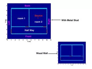
Back. Source. room 1. With Metal Stud. Right. room 2. Left. Hall Way. Front. Wood Wall. Simulation Configuration. Simulation Facts Grid resolution 1.0 cm; 1100x750 grids are used in XY plane. Time step 6.0e-11 sec. Radiation source is placed at the center of the right room.

Source
E N D
Presentation Transcript
Back Source room 1 With Metal Stud Right room 2 Left Hall Way Front Wood Wall
Simulation Configuration Simulation Facts • Grid resolution 1.0 cm; 1100x750 grids are used in XY plane. • Time step 6.0e-11 sec. Radiation source is placed at the center of the right room. • Scenario 1: Sinusoidal current source with f= 433 MHz. Jz Sin(2ft) for sec Then, switch to 0 for the rest time. Both with and without metal wall studs are simulated • Scenario 2: Sinusoidal current source with f= 433 MHz. Jz Sin(2ft) for sec Then, switch to 0 for the rest time. Both with and without metal wall studs are simulated Simulation Geometry • Two Rooms: 4mx4.5m each; • Wall • conductivity: 0.0005 S/m • Permittivity: 10 o • Thickness: 12 cm for inner wall; 20 cm for outer wall. • Wood Door • Conductivity: 0 S/m • Permittivity: 42 o • Cross-section: 90cmx6cm. • Metal Stud • Conductivity: 10^7 S/m • Permittivity: o • Cross-section: 5cmx8cm • Stud spacing: 30 cm • Otherwise: Vacuum • Conductivity: 0 S/m • Permittivity: o
Average Power Map (Sum and average) 433MHz Wood Wall 433MHz With metal Stud
Average Power Map 2.4GHz Wood Wall Metal Studs cause interference pattern. Leaking power is generally less for wall with metal studs. Leaking power for 2.4Ghz excitation is larger. 2.4 GHz With metal Stud
Detecting Emitted Signal and Estimating Distance Detect First Dip Delay for signal to subside
Wood Wall f = 433 MHz Wall with Studs f = 433 MHz Monitoring Points: We place monitoring points on 4 sides outside the wall: 0.5m to the wall, 1.0m apart. We record the arrival time of the first dip in the received signal at the monitoring point. Plots: The delay time dt is used to estimate the distance between the transmitter and receiver by using c x dt. In the above plots: We plot estimated distance vs. actual distance with color-coded symbols. The color represents the monitoring points on different sides as indicated in the legend. The blue line show the scenario if the estimated distance equals actual distance.
Wood Wall f = 2.4 GHz Wall with Studs f = 2.4 GHz Estimation error is different for monitoring at different sides. Estimation Errors due to multi-path propagation delay: F= 433 MHz: Wood Wall: Maximum Error=0.4m for distance=7.6m. Wall with metal studs: Maximum Error=0.9m for distance=8.3m. F=2.4 GHz: Wood Wall: Maximum Error=1.0m for distance=8.3m. Wall with metal studs: Maximum Error=1.4m for distance=8.3m. Error can be minimized by monitoring from optimized location and use magnitude info. (Stronger signal means closer to the source; near side is with less error.)