Download
1 / 23
230 likes | 265 Views
Learn about traditional search methods like Exhaustive Search, Greedy Algorithms, and Enumerating techniques for solving complex optimization problems efficiently. Understand the pros and cons of each method and how they can be applied in various scenarios.

E N D
MAE 552 – Heuristic Optimization Lecture 5 February 1 , 2002
Traditional Search Methods • Exhaustive Search checks each and every solution in the search space until the solution has been found. • Works well and is easy to code for small search problem. • For large problems it is not practical • Recall that for the 50 city TSP there are 1062 possible tours • If to evaluate each tour took, .00001 seconds it would take >1045 years to evaluate them all !!!!!
Exhaustive Search Methods • Exhaustive Search requires only that all of the solutions be generated in some systematic way. • The order the solutions are evaluated is irrelevant because all of them have to be looked at. • The basic question is how can we generate all the solutions to a particular problem??
X1=T X1=F X2=T X2=F X2=T X2=F X3=T X3=F X3=T X3=F X3=T X3=F X3=T X3=F . . . Exhaustive Search Methods • For the SAT problem the structure of the problem may allow some solutions to be pruned so they do not have to be searched.
X1=T X1=F X2=T X2=F X2=T X2=F X3=T X3=F X3=T X3=F X3=T X3=F X3=T X3=F Exhaustive Search Methods • Pruning is possible if after examining the values of a few variables it is clear that the candidate is not optimal. If there was a clause in the SAT: Means x1 and x2 must be present
Exhaustive Search Methods • All the the branches with either x1 and x2 FALSE could be pruned without ever looking at x3 leaving a much smaller S X1=T X1=F X2=T X2=F X2=T X2=F X3=T X3=F X3=T X3=F X3=T X3=F X3=T X3=F • Each node is traversed in order in a Depth-First Search
1 3 2 5 4 Enumerating the TSP • For some problems, including the TSP you cannot simply generate all possible solutions as many will not be feasible. • For example in many TSP problems all of the cities are not ‘fully connected’ so generating random permutations will generate many invalid solutions.
1 3 2 5 4 Enumerating the TSP • The tour 1-2-3-4-5 would not be valid for instance • Possibilities include penalized invalid candidates. • Generating new candidates by swapping adjacent pairs.
Enumerating the NLP • It is not strictly possible to enumerate all the possible candidates in a continuous problem (infinite number of solutions). • Continuous domain can be divided into a finite number of intervals. • There can be multiple levels to the enumeration. X2 X1
Enumerating the NLP • Step 1: Evaluate the center of each cell. X2 X1 • Step 2:Take the best cell and re-subdivide it.
Enumerating the NLP • There are several disadvantages to enumerating an NLP problem. • In order to really cover the design space the granularity of the cells must be very fine. • A coarse granularity of the cells increases the probability that the best solution will not be discovered i.e., the cell that contains the best solution wouldn’t show up because the level was too coarse. • When there are a large number of variables this become impractical. • If n=50 and each x were divided into 100 intervals yields 10100 cells!!!
Greedy Algorithms • Greedy algorithms attack a problem by constructing the complete solution in a series of steps. • The general idea is to assign the values for all of the decision variables one at a time. • At each step, the algorithm makes the best available decision, the ‘best’ profit, making it ‘greedy’. • Unfortunately making the best decision at each step does not necessarily result in the best solution overall.
Greedy Algorithms and the SAT • A simple greedy algorithm for the SAT problem is as follows: • For each variable from 1 to n, in any order,, assign the truth value that results in satisfying the greatest number of currently unsatisfied clauses. If there’s a tie, choose one of the best options at random. • At every step this greedy algorithm tries to satisfy the largest number of unsatisfied clauses. Example: • Starting with x1 set x1=TRUE as this will satisfy 3 clauses. • Unfortunately the first clause can never be satisfied with x1=TRUE
Greedy Algorithms and the SAT • There are heuristics that can be applied to improve this simple greedy algorithm. • It fails because it does not consider the variables in the right order. • If we started with the variables that occur in only a few clauses, x2, x3, x4+ leaving more commonly occurring variables for later. • The improved greedy algorithm could then be as follows: • 1. Sort the variables on the basis of there frequency, from the smallest to the largest. • 2. For each variable taken in the above order assign a value that would satisfy the greatest number of unsatisfied clauses.
Greedy Algorithms and the SAT • Now consider the following SAT • Where Z does not contain x1or x2 but contains numerous instances of the other variables. • Thus x1 is present in 3 clauses, x2 in four clauses and the other variables occur with higher frequency. • The improved greedy algorithm would assign x1 a value of TRUE because it satisfies 2 clauses and x2 a values of TRUE because it satisfies an additional 2 clauses which would violate the third and fourth clauses and the algorithm would fail.
Greedy Algorithms and the SAT • You could assign additional heuristics that would improve the greedy algorithm. • Unfortunately there would always be SAT problems that it could not solve. • If fact, there is no GREEDY algorithm that works for all SAT problems.
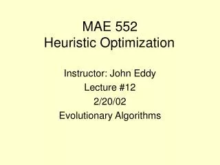
Greedy Algorithms and the TSP • For the travelling salesman problem (TSP), the most intuitive greedy algorithm is as follows. • Starting from a random city, proceed to the nearest unvisited city until every city has been visited, then return to the starting city. B 3 2 7 4 A C 5 D 23
B 3 2 7 4 A C 5 D 23 Greedy Algorithms and the TSP • Starting from Point A and applying the greedy algorithm the resultant tour is A-B-C-D Cost=2+3+23+5=33 Can we find a better tour?
B 3 2 7 4 A C 5 D 23 Greedy Algorithms and the TSP • By inspection A-C-B-D-A costs only 4+3+7+5=19 which is much better than that found by the greedy algorithm. • Once again you can think of other heuristics that would improve the performance of the greedy algorithm for certain cases, but you can always find a counter example in which it will fail
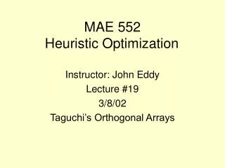
Greedy Algorithms and NLP • For the NLP a greedy algorithm would consider one variable at a time. • Start by choosing a random point. Change x1 until the objective function reaches an optimum with respect to it. • New point = Minimum F(x1, x2,..xn) with x2..xn held constant. • Hold x1 and x3..xn constant and optimize with respect to x2. • Repeat for all x’s. • This algorithm works fine if there are no interaction between design variables. • It is basically a series of line searches.
Greedy Algorithms and NLP For simple problems greedy algorithms can be effective.
Greedy Algorithms and NLP For mutimodal problems greedy algorithms are less effective
Greedy Algorithms • Greedy methods, whether applied to NLP, SAT, TSP, and many other domains are conceptually simple. • They make the best available move considering only a portion of the problem. • Unfortunately they pay for their simplicity by failing to provide good solutions to problems with interacting parameters. • These are the problems most commonly faced by designers.