Download
1 / 21
220 likes | 660 Views
Chapter 4: Motion in 2 and 3 dimensions. Chapter 4 Goals:. To introduce the concepts and notation for vectors: quantities that, in a single package, convey magnitude and direction motion To generalize our 1d kinematics to higher numbers of dimensions, using vector notation

E N D
Chapter 4: Motion in 2 and 3 dimensions Chapter 4 Goals: • To introduce the concepts and notation for vectors: quantities that, in a single package, convey magnitude and direction motion • To generalize our 1d kinematics to higher numbers of dimensions, using vector notation • To generalize Newtonian dynamics using vectors • To appreciate the glory of the Free Body Diagram and how it enables one to utilize N2 • To discuss projectile motion, and motion on a curve
Polar coordinates in 2 dimensions • (x,y) are the cartesian coordinates • two numbers needed to specify full information • convention for q is to start along x and swing counterclockwise The position of a point r hypotenuse x adjacent y opposite
Polar coordinates in 2 dimensions r hypotenuse x adjacent y opposite h o a
The displacement vector: we move into a higher dimension at last! • initial position is ri • final position is rf • displacement is Dr:= rf – ri y Dr rf x • Notice : the positions are origin-dependent, but the displacement is not!! ri • If it behaves like the displacement vector, then it is a vector!! It is the ‘paradigmatic’ vector. • vector subtraction is a bit tricky
Obvious language for vectors in two dimensions: magnitude and direction • magnitude of A: written |A| (some books say A) • it is just the length of A • |A| is always positive or 0 • technically it is not a scalar but don’t worry about that • |A| carries the units of A y A \A\ qA x • direction of A: written qA • usually counterclockwise from x axis • units of qA are degrees or radians
Pros of magnitude-direction language • we can writeA = {|A|,qA} • lends itself to obvious pictures • can easily be converted to compass (map) language: East x, and North y • addition and subtraction of vectors is done pictorially Cons of magnitude-direction language • accuracy of pictorial addition and subtraction is limited to human ability • laws of sines and cosines needed to calculate: messy • only convenient in 2d!! 3d requires the dreaded spherical trigonometry because there are 2 angles!!
Triangle method for adding vectors • A (and B) are two displacement vectors with B following A • magnitude : |A| or A • direction: an angle q, just like in previous figure • A is followed by B, to give resultantR = A + B • ‘tip-to-tail’ triangle method of adding vectors • One can just keep going, tip to tail style
Rules for adding vectors (and to multiply by scalar) • A + B = B + A: vector addition is commutative • (A + B) + C = A + (B + C): vector addition is associative • the negative of a vector is – A: same length as A but opposite direction [additive inverse] • There is a zero vector (no length) • vectors carry units and when added units mus be the same • ‘tip-to-tail’ triangle method of addition • cA: also a vector (opposite direction) if c<0 but ‘rescaled’ in length: |cA| = |c| |A|
How to subtract one vector from another • A – B := A + (– B): to subtract, just add the additive inverse • put both A and B tail-to-tail: then C = A – B has its tail at the tip of B (the one subtracted) and has its tip at the tip of A (the one added) • it seems to ‘start’ at B and end at A • This procedure is extremely important when finding changes in vectors!!! • Example:the displacement vector is precisely the change in the position vector!! {show Active Figure AF_0306
Addition Example : Taking a Hike A hiker begins a trip by first walking 25.0 km southeast from her car. She stops and sets up her tent for the night. On the second day, she walks 40.0 km in a direction 60.0° north of east, at which point she discovers a forest ranger’s tower. • Using ruler and protractor, lay out the two displacements A and B. Then, with the same tools, measure and then
A different and more flexible language: components • draw vector with tail at origin: • standard position y Ax • “drop a perpendicular” from tip to either Cartesian axis • you have made a right triangle A Ay qA |A| x • in this sketch, qA is larger than 90 but you can deal… • |A| is the hypotenuse; |A| ≥ 0 • Ax is the adjacent and here < 0 • Ay is the opposite and here > 0 • we write A = < Ax , Ay >
Converting from magnitude-angle to components Converting from magnitude-angle to components • This assumes that the angle is defined as ccw from x axis {show Active Figure AF_0303} Pros of component language • addition and subtraction of two (or more) vectors is simplicity itself: just add (subtract) the components like scalars and the resultant vector‘s (difference vector’s) components are known!
Revisiting the vector addition example Section 3.4
Finishing the Example • Now we would work back from component language to magnitude-angle language: • ‘net displacement is 41.3 km, at a bearing of 65.9° East of North’ • R = {41.3 km, 24.1°} Section 3.4
A third language that uses components: unit vectors • i is a vector of unit length, with no units, that points along x • j and k are similar, along y (and z) • create the vectors i Ax & j Ay i Ax y A j Ay |A| x qA • A truly explicit way to write A • remember: |i| = |j| = |k| = 1 • (no units, and but one unit long!!)
What other operations can we do with vectors? • cannot divide by a vector; vectors are only ‘upstairs’ • dot (scalar (inner)) product of two • cross (vector (outer (wedge))) product of two • we can take their derivative with respect to a scalar • we can integrate them but usually we integrate some kind of scalar product… The scalar product of two vectors • put them tail-to-tail, with q the angle between (0° ≤ q ≤ 180°) A q • the result is indeed a scalar • A∙B = B ∙A (commutative) B
More about the scalar product • a measure of the parallelness of the vectors, as well as the magnitudes • A∙B = (|A|)(|B| cos q) = length of A times the length of B’s projection along the line of A • A∙B = (|B|)(|A| cos q) = length of B times the length of A’s projection along the line of B • A∙A = |A|2 • i∙i = j∙j = k∙k =1 i∙j = j∙k = 0 etc. • a vector’s component in a certain direction is the scalar product of that vector with a unit vector in that direction: Cn = C∙n • [to make a unit vector, just divide a vector by its magnitude: a = A/|A| ]
Kinematics in ‘higher dimensions’ I: position and displacement as vector • position is now a vector: • the three components of the position: r:= <x, y, z> • if the arena is 2d, drop the z-stuff • displacement is change in position: Dr = rB – rA or Dr = rf – ri or, best of all, Dr = r(t+Dt) – r(t) • it is a vector with tail at r(t) and tip at r(t+Dt) • displacement vector not usually drawn in standard position but may be, especially if you are adding a second displacement to the first and you don’t really care about ‘initial’ position, or you take that to be zero • the displacement vector is origin-independent!
Kinematics in ‘higher dimensions’ II: the (instantaneous) velocity vector • velocity is now a vector: • here we used the fact that the unit vectors do not vary with time as the body moves around • the three components of the velocity v:= <vx, vy , vz > where vx(t)=dx(t)/dt and similarly for y and z
Kinematics in ‘higher dimensions’ III • how do we understand this? • start with average velocity: of course, <v> = Dr/Dt Dr(t) y r(t) path of object r(t+Dt) x • <v> is a vector: it’s a vector (Dr) times a number (1/Dt) • magnitude: |<v>| = | Dr |/|Dt| • direction: same as direction of Dr
Kinematics in ‘higher dimensions’ IV • we now let Dt get really small (Dt 0) and call it dt • as that shrinks, so does Dr : call it dr Dr(t) y dr(t) r(t+dt) r(t) r(t+Dt) path of object x • magnitude: |v| = |dr |/dt| = speed • direction: tangent to the path in space!!!