Contents
230 likes | 244 Views
This article explores various non-linear functions, such as quadratic, cubic, reciprocal, and exponential functions, and how their graphs can be transformed through translations, reflections, and stretches. It also covers the concept of function notation.

Contents
E N D
Presentation Transcript
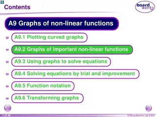
A9 Graphs of non-linear functions Contents A9.1 Plotting curved graphs • A • A A9.3 Using graphs to solve equations • A A9.2 Graphs of important non-linear functions A9.4 Solving equations by trial and improvement • A A9.5 Function notation • A A9.6 Transforming graphs • A
Quadratic functions y = –3x2 y = x2 y = x2 – 3x A quadratic function always contains a term in x2. It can also contain terms in x or a constant. Here are examples of three quadratic functions: The characteristic shape of a quadratic function is called a parabola.
Cubic functions y = x3– 4x y = x3+ 2x2 A cubic function always contains a term in x3. It can also contain terms in x2 or x or a constant. Here are examples of three cubic functions: y = -3x2– x3
Reciprocal functions y = y = y = –4 3 x x 1 x A reciprocal function always contains a fraction with a term in x in the denominator. Here are examples of three simple reciprocal functions: In each of these examples the axes form asymptotes. The curve never touches these lines.
Exponential functions y = 2x y = 3x y = 0.25x An exponential function is a function in the form y = ax, where a is a positive constant. Here are examples of three exponential functions: In each of these examples, the x-axis forms an asymptote.
The equation of a circle y r y x 0 x One more graph that you should recognize is the graph of a circle centred on the origin. We can find the relationship between the x and y-coordinates on this graph using Pythagoras’ theorem. (x, y) Let’s call the radius of the circle r. We can form a right angled triangle with length y, height x and radius r for any point on the circle. Using Pythagoras’ theorem this gives us the equation of the circle as: x2 + y2 = r2
A9 Graphs of non-linear functions Contents A9.1 Plotting curved graphs • A A9.2 Graphs of important non-linear functions • A A9.3 Using graphs to solve equations • A A9.6 Transforming graphs A9.4 Solving equations by trial and improvement • A A9.5 Function notation • A • A
Transforming graphs of functions Graphs can be transformed by translating, reflecting, stretching or rotating them. The equation of the transformed graph will be related to the equation of the original graph. When investigating transformations it is most useful to express functions using function notation. For example, suppose we wish to investigate transformations of the function f(x) = x2. The equation of the graph of y = x2, can be written as y = f(x).
Vertical translations x The graph of y = f(x) + a is the graph of y = f(x) translated by the vector . 0 a Here is the graph of y = x2, where y = f(x). This is the graph of y = f(x) + 1 y and this is the graph of y = f(x) + 4. What do you notice? This is the graph of y = f(x) – 3 and this is the graph of y = f(x) – 7. What do you notice?
Horizontal translations x The graph of y = f(x + a) is the graph of y = f(x) translated by the vector . –a 0 Here is the graph of y = x2 – 3, where y = f(x). This is the graph of y = f(x – 1), y and this is the graph of y = f(x – 4). What do you notice? This is the graph of y = f(x + 2), and this is the graph of y = f(x + 3). What do you notice?
Reflections in the x-axis x The graph of y = –f(x) is the graph of y = f(x) reflected in the x-axis. Here is the graph of y = x2 –2x – 2, where y = f(x). y This is the graph of y = –f(x). What do you notice?
Reflections in the y-axis x The graph of y = f(–x) is the graph of y = f(x) reflected in the y-axis. Here is the graph of y = x3 + 4x2 – 3 where y = f(x). y This is the graph of y = f(–x). What do you notice?
Stretches in the y-direction The graph of y = af(x) is the graph of y = f(x) stretched parallel to the y-axis by scale factor a. Here is the graph of y = x2, where y = f(x). This is the graph of y = 2f(x). y What do you notice? This graph is is produced by doubling the y-coordinate of every point on the original graph y = f(x). This has the effect of stretching the graph in the vertical direction. x
Stretches in the x-direction x The graph of y = f(ax) is the graph of y = f(x) stretched parallel to the x-axis by scale factor . 1 a Here is the graph of y = x2 + 3x – 4, where y = f(x). This is the graph of y = f(2x). y What do you notice? This graph is is produced by halving the x-coordinate of every point on the original graph y = f(x). This has the effect of compressing the graph in the horizontal direction.