Download

1 / 19
210 likes | 587 Views
Accelerated Stability Modeling for Bioproducts. 2013 MBSW, Muncie, Indiana May 21, 2013 Kevin Guo. Examples of Bioproducts. Amgen/Pfizer. Eli Lilly. Genentech. Genentech. Genentech. Merck. Abbott Labs. Eli Lilly. What is Bioproduct.

E N D
Accelerated Stability Modeling for Bioproducts 2013 MBSW, Muncie, Indiana May 21, 2013 Kevin Guo
Examples of Bioproducts Amgen/Pfizer Eli Lilly Genentech Genentech Genentech Merck Abbott Labs Eli Lilly
What is Bioproduct Bioproducts are proteins produced from recombinant DNA and grown in an expression system such as bacteria, yeast, or eukaryotic systems
Background • One of the key objectives in developing bioproduct is to find a commercial formulation prototype that has an acceptable stability profile throughout a desired shelf-life of 18 months or more, under typical storage condition of 2-8°C • To expedite the decision process of selecting the optimal formulation prototype, a short-term accelerated stability is usually conducted by subjecting the formulation candidates to elevated multi temperature exposures (typically 15°C and higher) • Based on this short-term multi temperature stability study, a prediction model is then developed to estimate the long-term stability profile of the formulation candidates under the intended long-term storage condition
Why Stability Testing • Safety point of view from patient • Critical quality attribute (CQA) • Establish shelf life of the drug • Study the storage conditions • Study the container closure system • Provide evidence how the quality of the drug product changes over time
What’s so Special about Bioproduct Stability? Common problems with stability of proteins • Usually sensitive to light, heat, air, and trace metal impurities • Small or large stress factors can disrupt protein folding • Numerous physical degradation routes, including agitation, freezing, interaction with surfaces and phase boundaries • Possible Non-Arrhenius behavior • One type of degradation can facilitate other types of degradation leading to a cascading effect • Possibility of different degradation mechanisms appearing depending on the age of the product • Limited formulation options Reference: Handbook of Stability Testing in Pharmaceutical Development. Anthony Mazzeo and Patrick Carpenter, Ch17, Stability Studies for Biologics
Bioproduct Stability • Why accelerated stability studies work despite the problems listed on the previous slide? • Degradation is often reasonably Arrhenius below 40°C • Information from pre-formulation studies and other one-off studies
Challenges in Accelerated Stability Modeling • When developing the prediction model from the short-term accelerated stability study: • Bioproducts typically degrade in a nonlinear fashion, numerous chemical degradation routes possible, much more so than the small molecule compounds • The underlying degradation mechanism is often very complex and a characterization study to understand the degradation kinetic is prohibitively expensive • Limited resources to execute the accelerated study that minimal number of temperatures and testing time-points can be incorporated in the study design • This presentation describes a proposal on how to develop the prediction model. Some key features: • Leveraging Arrhenius principle of the temperature dependence of a chemical reaction
Accelerated Stability Study Design • Key features of the stability design • Short-term, should be completed in 3 months or less • Typically utilize 4 temperatures at minimum: long-term storage condition of 5°C + 3 elevated temperatures (15 – 40°C) • Highest temperature is chosen such that it is representative of lower temperature stability profiles (e.g. elevated temperature degrades in the same pathway as the lower ones) • Utilize materials (e.g. Drug Substance) that are representative of those for commercial use • May incorporate other factors of interests besides temperature (e.g. pH, concentration of drug substance, choice of excipient, etc)
Fixed Time-points vs. Fixed Amt of Change • Fixed Schedule • Advantages: • platform-wide approach (doesn’t need to vary with molecule) • requires little prior knowledge • provides stability profile • Disadvantages: • labor intensive • different levels of degradation at different storage conditions – can bias rate coefficient estimates Months • Fixed Degradant • Advantages: • efficient • same level of degradation (rate coefficient bias does not depend on storage condition) • Disadvantages: • requires Ea estimate to design correct storage temperature / time-point combinations • target degradant level must be selected a-priori Months
Arrhenius Equation • Rate constant k of a chemical reaction depends on the temperature (Kelvin) and activation energy Ea according to the following equation: k = Reaction rate Ea = Activation Energy (Kcal mol-1) R = Gas constant (Kcal mol-1 K-1) T = Temperature in Kelvin kR,0 = Pre-exponential Factor
Double Regression Analysis • Step 1. Estimation of the k • Fit “Zero-order” regression of the concentration of an analytical property vs. time, at each Temperature condition • Step 2. Estimation of the Activation Energy • Fit Arrhenius Regression, using fitted k(T) values [i.e., slopes] from regression in Step 1 as Ys:
Double Regression Analysis • High variability relative to degradation may lead to negative rate constant estimates that become truncated at the logarithm scale (e.g. increasing monomer ln(-x)=NA) • Insufficient resolution (high degree of rounding) that results in the same value at each time-point can produce zero rate constant estimates (k=0) that become truncated (ln(0) -inf) • Non-constant variance with the logarithmic form of Arrhenius
Non-Linear Model Description Therapeutic proteins are complex molecules that can degrade (aggregate) via a variety of different physical/chemical mechanisms. reactive For simplicity, consider only two broad categories: non-reactive time Only the ‘reactive’ monomer aggregates Use first-order Arrhenius kinetics to describe the system Parameters: Mtotal – total monomer concentration t – time MNR – non-reactive monomer concentration MR,0 – reactive monomer concentration at t = 0 kR– first-order rate constant kR,0– Arrhenius pre-exponential term Ea – apparent activation energy kR,0’ = ln( kR,0 ) – for numerical convergence A good compromise between first-principles rigor and practical limitations
Non-Linear Model Fitting MNR + MR,0 MNR Mtotal time a Formulation = unique set of pH, ionic strength, excipients; replicates of a given formulation (different “runs”) were fit independently. Parameters: Mtotal – total monomer concentration t – time MNR – non-reactive monomer concentration MR,0 – reactive monomer concentration at t = 0 kR– first-order rate constant kR,0– Arrhenius pre-exponential term Ea – apparent activation energy kR,0’ = ln( kR,0 ) – for numerical convergence The nonlinear regression platform in JMP 8.0.2 was used to estimate unknown parameters
Double Regression vs. Non-Linear 99 TempC 98 5 25 97 r 30 e 96 m 40 o n 95 o M 94 93 92 91 0 1 2 3 Nonlinear Model Double Regression Month 1 99 0.5 98 100 0 ) 97 K ( -0.5 r 98 e n 96 m r L -1 e o 96 m n -1.5 95 o o M n -2 o 94 94 M -2.5 2 3 4 5 6 93 92 3 3 3 3 3 0 0 0 0 0 0 0 0 0 0 92 . . . . . 0 0 0 0 0 90 91 1/T 1 2 3 0 0 1 2 3 Month Month Ea=15.486
Concluding Remarks • Summary • An approach for modeling the accelerated stability data for biomolecules are presented • The nonlinear model based on the interplay between of reactive and non-reactive species shown to fit the data quite well when there is sufficient degradation • Future work • Evaluate alternative loss functions for better model selection (i.e. goodness-of-fit) • Evaluate alternative nonlinear models • Find potential patterns from existing biomolecules that may provide clues on how to better design and analyze data for future studies
Acknowledgments • Adam Rauk, inVentiv Health • Will Weiss • Suntara Cahya