Download
1 / 22
220 likes | 374 Views
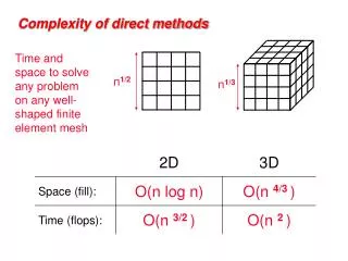
n 1/2. n 1/3. Complexity of direct methods. Time and space to solve any problem on any well-shaped finite element mesh. n 1/2. n 1/3. Complexity of linear solvers. Time to solve model problem (Poisson ’ s equation) on regular mesh. Hierarchy of matrix classes (all real).

E N D
n1/2 n1/3 Complexity of direct methods Time and space to solve any problem on any well-shaped finite element mesh
n1/2 n1/3 Complexity of linear solvers Time to solve model problem (Poisson’s equation) on regular mesh
Hierarchy of matrix classes (all real) • General nonsymmetric • Diagonalizable • Normal • Symmetric indefinite • Symmetric positive (semi)definite = Factor width n • Factor width k . . . • Factor width 4 • Factor width 3 • Symmetric diagonally dominant = Factor width 2 • Generalized Laplacian = Symmetric diagonally dominant M-matrix • Graph Laplacian
Definitions • The Laplacian matrix of an n-vertex undirected graph G is the n-by-n symmetric matrix A with • aij = -1 if i ≠ j and (i, j) is an edge of G • aij = 0 if i ≠ j and (i, j) is not an edge of G • aii = the number of edges incident on vertex i • Theorem: The Laplacian matrix of G is symmetric, singular, and positive semidefinite. The multiplicity of 0 as an eigenvalue is equal to the number of connected components of G. • A generalized Laplacian matrix (more accurately, a symmetric weakly diagonally dominant M-matrix) is an n-by-n symmetric matrix A with • aij≤ 0 if i ≠ j • aii≥Σ |aij| where the sum is over j ≠ i
Edge-vertex factorization of generalized Laplacians • A generalized Laplacian matrix A can be factored as A = UUT, where U has: • a row for each vertex • a column for each edge, with two nonzeros of equal magnitude and opposite sign • a column for each excess-weight vertex, with one nonzero A = U × UT excess-weightvertices(1nz/col) vertices vertices vertices edges(2 nzs/col) vertices
Support Graph Preconditioning • CFIM: Complete factorization of incomplete matrix • Define a preconditioner B for matrix A • Explicitly compute the factorization B = LU • Choose nonzero structure of B to make factoring cheap (using combinatorial tools from direct methods) • Prove bounds on condition number using both algebraic and combinatorial tools +: New analytic tools, some new preconditioners +: Can use existing direct-methods software -: Current theory and techniques limited
Spanning Tree Preconditioner [Vaidya] • A is generalized Laplacian(symmetric diagonally dominant with negative off-diagonal nzs) • B is the gen Laplacian of a maximum-weight spanning tree for A (with diagonal modified to preserve row sums) Form B: costs O(n log n) or less time (graph algorithms for MST) Factorize B = RTR: costs O(n) space and O(n) time (sparse Cholesky) Apply B-1: costs O(n) time per iteration G(A) G(B)
Combinatorial analysis: cost of preconditioning • A is generalized Laplacian(symmetric diagonally dominant with negative off-diagonal nzs) • B is the gen Laplacian of a maximum-weight spanning tree for A (with diagonal modified to preserve row sums) • Form B: costsO(n log n) time or less (graph algorithms for MST) • Factorize B = RTR: costs O(n) space and O(n) time (sparse Cholesky) • Apply B-1: costs O(n) time per iteration (two triangular solves) G(A) G(B)
Numerical analysis: quality of preconditioner • support each edge of A by a path in B • dilation(A edge) = length of supporting path in B • congestion(B edge) = # of supported A edges • p = max congestion, q = max dilation • condition number κ(B-1A) bounded by p·q (at most O(n2)) G(A) G(B)
Spanning Tree Preconditioner [Vaidya] • can improve congestion and dilation by adding a few strategically chosen edges to B • cost of factor+solve is O(n1.75), or O(n1.2) if A is planar • in experiments by Chen & Toledo, often better than drop-tolerance MIC for 2D problems, but not for 3D. G(A) G(B)
Numerical analysis: Support numbers Intuition from networks of electrical resistors: • graph = circuit; edge = resistor; weight = 1/resistance = conductance • How much must you amplify B to provide as much conductance as A? • How big does t need to be for tB – A to be positive semidefinite? • What is the largest eigenvalue of B-1A ? The support of B for A is σ(A, B) = min { τ : xT(tB– A)x 0 for all x and all t τ } • If A and B are SPD then σ(A, B) = max{λ : Ax = λBx} = λmax(A, B) • Theorem: If A and B are SPD then κ(B-1A) = σ(A, B) · σ(B, A)
Old analysis, splitting into paths and edges • Split A = A1+ A2 + ··· + Ak and B = B1+ B2 + ··· + Bk • such that Ai and Bi are positive semidefinite • Typically they correspond to pieces of the graphs of A and B (edge, path, small subgraph) • Theorem: σ(A, B) maxi {σ(Ai , Bi)} • Lemma: σ(edge, path) (worst weight ratio) · (path length) • In the MST case: • Ai is an edge and Bi is a path, to give σ(A, B) p·q • Bi is an edge and Ai is the same edge, to give σ(B, A) 1
Edge-vertex factorization of generalized Laplacians • A generalized Laplacian matrix A can be factored as A = UUT, where U has: • a row for each vertex • a column for each edge, with two nonzeros of equal magnitude and opposite sign • a column for each excess-weight vertex, with one nonzero A = U × UT excess-weightvertices(1nz/col) vertices vertices vertices edges(2 nzs/col) vertices
New analysis: Algebraic Embedding Lemma vv[Boman/Hendrickson] Lemma: If V·W=U, then σ(U·UT, V·VT) ||W||22 (with equality for some choice of W) Proof: • take t ||W||22 = λmax(W·WT) = max y0 { yTW·WTy / yTy } • then yT (tI - W·WT) y 0 for all y • letting y = VTx gives xT (tV·VT - U·UT) x 0 for all x • recall σ(A, B) = min{τ : xT(tB– A)x 0 for all x, all t τ} • thus σ(U·UT, V·VT) ||W||22
[ ] a2 +b2-a2 -b2 -a2 a2 +c2 -c2-b2 -c2 b2 +c2 [ ] a2 +b2-a2 -b2 -a2 a2 -b2 b2 B =VVT A =UUT ] [ ] [ ab-a c-b ab-a c-b-c U V -a2 -c2 -a2 -b2 -b2
[ ] a2 +b2-a2 -b2 -a2 a2 +c2 -c2-b2 -c2 b2 +c2 [ ] a2 +b2-a2 -b2 -a2 a2 -b2 b2 B =VVT A =UUT ] [ ] ] [ [ 1-c/a1 c/b/b ab-a c-b ab-a c-b-c = x U V W -a2 -c2 -a2 -b2 -b2 A edges B edges
[ ] a2 +b2-a2 -b2 -a2 a2 +c2 -c2-b2 -c2 b2 +c2 [ ] a2 +b2-a2 -b2 -a2 a2 -b2 b2 B =VVT A =UUT ] [ ] ] [ [ 1-c/a1 c/b/b ab-a c-b ab-a c-b-c = x U V W -a2 -c2 -a2 -b2 -b2 σ(A, B) ||W||22 ||W||x ||W||1 = (max row sum) x (max col sum) (max congestion) x (max dilation) A edges B edges
Extensions, remarks, open problems I • Using another matrix norm inequality [Boman]: ||W||22 ||W||F2= sum(wij2) = sum of (weighted) dilations, and [Alon, Karp, Peleg, West]construct spanning trees with average weighted dilation exp(O((log n loglog n)1/2)) = o(n ). This gives condition number O(n1+) and solution time O(n1.5+),compared to Vaidya’sO(n1.75) with augmented MST. • Is there a graph construction that minimizes ||W||22directly? • [Spielman, Teng]: complicated recursive partitioning construction with solution time O(n1+) for all generalized Laplacians! (Uses yet another matrix norm inequality.)
Extensions, remarks, open problems II • Make spanning tree methods more effective in 3D? • Vaidya gives O(n1.75) in general, O(n1.2) in 2D. • Issue: 2D uses bounded excluded minors, not just separators. • Support theory methods for more general matrices? • [Boman, Chen, Hendrickson, Toledo]: different matroid for all symmetric diagonally dominant matrices (= factor width 2). • Matrices of bounded factor width? Factor width 3? • All SPD matrices? • Is there a version that’s useful in practice? • Maybe for non-geometric graph Laplacians? • [Koutis, Miller, Peng 2010] simplifies Spielman/Teng a lot. • [Kelner et al. 2013]: random Kaczmarz projections in the dual space – even simpler, good O() theorems, but not yet fast enough in practice.
B has positive (dotted) edges that cancel fill B has same row sums as A Strategy: Use the negative edges of B to support both the negative edges of A and the positive edges of B. -1 -1 -1 -1 -1 -1 -1 -1 -1 -1 -1 -1 -1 -1 -1 -1 -1 -1 -1 -1 -1 -1 -1 -1 -1 -1 -1 -1 -1 -1 -1 -1 -1 -1 -1 -1 -1 -1 -1 -1 -1 -1 -1 -1 -1 -1 -1 -1 B A .5 .5 .5 .5 .5 .5 .5 .5 .5 A = 2D model Poisson problem B = MIC preconditioner for A Support-graph analysis of modified incomplete Cholesky
Every dotted (positive) edge in B is supported by two paths in B Each solid edge of B supports one or two dotted edges Tune fractions to support each dotted edge exactly 1/(2n – 2) of each solid edge is left over to support an edge of A Supporting positive edges of B
Analysis of MIC: Summary • Each edge of A is supported by the leftover 1/(2n – 2) fraction of the same edge of B. • Therefore σ(A, B) 2n – 2 • Easy to show σ(B, A) 1 • For this 2D model problem, condition number is O(n1/2) • Similar argument in 3D gives condition number O(n1/3) or O(n2/3) (depending on boundary conditions)