Structure solution by Direct Methods
Structure solution by Direct Methods. Carmelo Giacovazzo Istituto di Cristallografia, CNR, Bari University, Italy carmelo.giacovazzo@ic.cnr.it.


Structure solution by Direct Methods
E N D
Presentation Transcript
Structure solution by Direct Methods Carmelo Giacovazzo Istituto di Cristallografia, CNR, Bari University, Italy carmelo.giacovazzo@ic.cnr.it
Let us answer the following questions:crystal structure ? crystal structure ? As a consequence:
O Xo O’ rj rj’ A third question: structure
A fourth basic questionHow can we derive phases from diffraction moduli? This seems contradictory: indeed Phase values depend on the origin chosen by the user, moduli are independent of the user .The moduli are structure invariants, the phases are not structure invariants.Evidently, from the moduli we can derive information only on those combinations of phases ( if they exist) which are structure invariants.
The simplestinvariant : the tripletinvariantUse the relation F’h = Fhexp ( -2ihX0) tocheckthat the invariantFhFkF-h-kdoesnotdepend on the origin.The sum (h + k+-h-k ) iscalledtripletphaseinvariant .
Structure invariantsAny invariant satisfies the condition that the sum of the indices is zero:doublet invariant : Fh F-h = | Fh|2triplet invariant : Fh Fk F-h-kquartet invariant :Fh Fk Fl F-h-k-lquintet invariant : Fh Fk Fl Fm F-h-k-l-m
r2 r1 a2 a1 The prior informationwe can use for deriving the phase estimates may be so summarised:1) atomicity: the electron density is concentrated in atoms:2) positivity of the electron density:( r ) > 0 f > 03) uniform distribution of the atoms in the unitcell.
The Wilson statistics • Under the above conditions Wilson ( 1942,1949) derived the structure factor statistics. The main results where: • (1) • Eq.(1) is : • a) resolution dependent (fj varies with θ ), • b) temperature dependent: • From eq.(1) the concept of normalized structure factor arises:
The Wilson Statistics • |E|-distributions: and in both the cases. The statistics may be used to evaluate the average themel factor and the absolute scale factor.
A s2 Fh0 A x y
The Cochran formulah,k =h + k + -h-k = h + k - h+kP(hk) [2 I0]-1exp(G cos hk)where G = 2 | Eh Ek Eh+k |/N1/2Accordingly:h + k - h+k 0 G = 2 | Eh Ek Eh+k |/N1/2 h - k - h-k 0 G = 2 | Eh Ek Eh-k |/N1/2h k - h-k G = 2 | Eh Ek Eh-k |/N1/2
The tangent formulaA reflection can enter into several triplets.Accordinglyh k1 + h-k1 = 1with P1(h) G1 = 2| Eh Ek1 Eh-k1 |/N1/2h k2 + h-k2 = 2 with P2(h) G2 = 2| Eh Ek2 Eh-k2 |/N1/2……………………………………………………………………………………………………….h kn + h-kn = n with Pn(h) Gn = 2| Eh Ekn Eh-kn |/N1/2Then P(h) j Pj(h) L-1 j exp [Gj cos (h - j )] = L-1 exp [ cos (h - h )]where
The random starting approachTo apply the tangent formula we need to know one or more pairs ( k + h-k ). Where to find such an information?The most simple approach is the random starting approach. Random phases are associated to a chosen set of reflections. The tangent formula should drive these phases to the correct values. The procedure is cyclic ( up to convergence).How to recognize the correct solution?Figures of meritcan or cannot be applied
Tangent cycles • φ1 φ’1 φ’’1 ……………. φc1 • φ2 φ’2 φ’’2 ……………. φc2 • φ3 φ’3 φ’’3 …………….. φc3 • …………………………………………………………………….. • φnφ’nφ’’n………………. φcn
Ab initio phasing • SIR2011 is able to solve -small size structures (up to 80 atoms in the a.u.); -medium-size structures ( up to 200); -large size (no upper limit) • It uses • Patterson deconvolution techniques • ( multiple implication transformations) • as well as • Direct methods • to obtain a starting set of phases. They are extended and refined via • electron density modification techniques
The VLD ( vive la difference) method • Historically, the difference Fourier synthesis is calculated via Fourier coefficients • In a modern way it is calculated via the coefficients • where m and D parameters take into account the correlation between model and target structure. • m=D=0 for uncorrelated model, m=D=1 for identical models.
According to our recent publication ( 2010) the best coefficient for a difference Fourier synthesis is : • That is , it is the sum of the classical coefficient • and of the flipping term • The flipping term is dominant when the model is poor, goes to zero when the model coincides with the target.
A difference Fourier synthesis calculated by such coefficient will have : • Big negative minima where the atoms of the model structure are in wrong position; • Medium positive maxima in correspondence of the atoms of the target structure which are not part of the model.
Stepsof VLD algorithm • ( Burla, Giacovazzo, Polidori, (2010), • J.Appl. Cryst. 43, 825-836) • A random E- electron density map is calculated. • The model structure is obtained by selecting 2.5% of the largest intensity pixels. • A difference electron density map is calculated via the best coefficients . • is modified ( by selecting 4% of the pixels with largest positive values and 4% of the pixels with largest negative values ) and added to to obtain a new estimate of :
The corresponding E-map is calculated which is submitted to cycles of EDM. In each cycle the parameter is updated. • At the end a new model is obtained and a next iteration starts.
Work in progress • We have combined VLD with RELAX. • RELAX is a procedure for shifting a model from a wrong into the correct position. • All the calculations are transparent for the user. • The results are below described.
SMALL STRUCTURES ( up to 80 atoms in the asymmetric unit • 33 test structures • Solution found in 7sec ( on average); • 1.1 seeds necessary for finding the solution.
On the medium size structures above mentioned: • <RES>= 0.16, • <T>= 4.6 mins, • <Δφ>=16°, • <seed>= 2.8
For the solved proteins ( 12 over 35 unsolved in default, 10 or less if we use a larger number of seeds): • <RES>=0.28, • <fFOM2>=3.75 • <T>=0.5 hours, • <Δφ>=21°, • <seed>=2.4