Download
1 / 22
220 likes | 367 Views
Measuring Center. Lecture 15 Sections 5.1 – 5.2 Tue, Feb 14, 2006. Measuring the Center. Often, we would like to have one number that that is “representative” of a population or sample.

E N D
Measuring Center Lecture 15 Sections 5.1 – 5.2 Tue, Feb 14, 2006
Measuring the Center • Often, we would like to have one number that that is “representative” of a population or sample. • It seems reasonable to choose a number that is near the “center” of the distribution rather than in the left or right extremes. • But there is no single “correct” way to do this.
Measuring the Center • Mean – the simple average of a set of numbers. • Median – the value that divides the set of numbers into a lower half and an upper half. • Mode – the most frequently occurring value in the set of numbers.
Measuring the Center • In a unimodal, symmetric distribution, these values will all be near the center. • In other-shaped distributions, they may be spread out.
The Mean • We use the letter x to denote a value from the sample or population. • The symbol means “add them all up.” • So, x means add up all the values in the population or sample (depending on the context). • Then the sample mean is
The Mean • We denote the mean of a sample by the symbolx, pronounced “x bar”. • We denote the mean of a population by , pronounced “mu” (myoo). • Therefore,
TI-83 – The Mean • Enter the data into a list, say L1. • Press STAT > CALC > 1-Var Stats. • Press ENTER. “1-Var-Stats” appears. • Type L1 and press ENTER. • A list of statistics appears. The first one is the mean. • See p. 301 for more details.
Examples • Use the TI-83 to find the mean of the data in Example 5.1(a), p. 301.
Weighted Means • Continuing the previous example, suppose we surveyed another group of households and found the following number of children: 3, 2, 5, 2, 6. • Find the average of this group by itself. • Combine the two averages into one average for all 15 households.
The Median • Median – The middle value, or the average of the middle two values, of a sample or population, when the values are arranged from smallest to largest. • The median, by definition, is at the 50th percentile. • It separates the lower 50% of the sample from the upper 50%.
The Median • When n is odd, the median is the middle number, which is in position (n + 1)/2. • Find the median of 3, 2, 5, 2, 6. • When n is even, the median is the average of the middle two numbers, which are in positions n/2 and n/2 + 1. • Find the median of 2, 3, 0, 2, 1, 0, 3, 0, 1, 4.
The Median • Alternately, we could calculate (n + 1)/2 in all cases. • If it is a whole number, then use that position. • If it is halfway between two whole numbers, take use both positions and take the average.
TI-83 – The Median • Follow the same procedure that was used to find the mean. • When the list of statistics appears, scroll down to the one labeled “Med.” It is the median. • Use the TI-83 to find the medians of the samples • 3, 2, 5, 2, 6 • 2, 3, 0, 2, 1, 0, 3, 0, 1, 4
The Median vs. The Mean • In the last example, change 4 to 4000 and recompute the mean and the median. • How did the change affect the median? • How did the change affect the mean? • Which is a better measure of the “center” of this sample?
The Mode • Mode – The value in the sample or population that occurs most frequently. • The mode is a good indicator of the distribution’s central peak, if it has one.
Mode • The problem is that many distributions do not have a peak or have several peaks. • In other words, the mode does not necessarily exist or there may be several modes.
Mean, Median, and Mode • If a distribution is symmetric, then the mean, median, and mode are all the same and are all at the center of the distribution.
Mean, Median, and Mode • However, if the distribution is skewed, then the mean, median, and mode are all different.
Mean, Median, and Mode • However, if the distribution is skewed, then the mean, median, and mode are all different. • The mode is at the peak. Mode
Mean, Median, and Mode • However, if the distribution is skewed, then the mean, median, and mode are all different. • The mode is at the peak. • The mean is shifted in the direction of skewing. Mean Mode
Mean, Median, and Mode • However, if the distribution is skewed, then the mean, median, and mode are all different. • The mode is at the peak. • The mean is shifted in the direction of skewing. • The median is (typically) between the mode and the mean. Mean Mode Median
1/2 x 0 4 Let’s Do It! • Let’s Do It! 5.6, p. 309 – A Different Distribution. • Do the same for the distribution