Download
1 / 30
300 likes | 449 Views
Market. MBA NCCU Managerial Economics Jack Wu. Case: tanker Service market , 2005. Impact of Increasing oil prices Increasing China imports More stringent tanker standards. Characteristics of Perfectly Competitive Market. homogeneous (identical) product many small buyers

E N D
Market MBA NCCU Managerial Economics Jack Wu
Case: tanker Service market, 2005 • Impact of • Increasing oil prices • Increasing China imports • More stringent tanker standards
Characteristics of Perfectly Competitive Market • homogeneous (identical) product • many small buyers • many small sellers • price takers (No influence on price) • free entry and exit (No barriers) • Both buyers and sellers share equal (symmetric) information
Differentiated or Homogeneous? • In market where products are differentiated, competition is not as keen as that in a market where products are homogeneous. • Compare • mineral water – differentiated • gold – pure commodity
No Market Power • Many small buyers • Many small sellers • Both buyers and sellers have no market powers. • Both buyers and sellers are price takers. • Note: buyer/seller with market power can influence market conditions
No barriers • Free entry and exit • No entry barriers to potential competitors • No exit barriers to existing sellers
Free Entry? Japanese Beer Market, pre-’94: Ministry of Finance • production licenses for minimum of 2 million liters a year • sales licenses limited to small family-owned stores
Symmetric or Asymmetric Information • Market with differences in information not as competitive as one where all buyers and sellers have equal information • Compare • photocopying service • medical treatment • legal advice
Market Equilibrium, I Price at which quantity demanded equals quantity supplied • when market out of equilibrium, market forces push price towards equilibrium
MARKET EQUILIBRIUM, II a excess supply supply Price ($ per ton-mile) 22 b 20 equilibrium c demand 0 8 10 11 Quantity (Million ton-miles a year)
Market Equilibrium, III • excess supply = excess of quantity supplied over quantity demanded • triggers price decrease • excess demand = excess of qty demanded over qty supplied • triggers price increase
Supply Shift, I • supply shifts down (right) -> lower price, larger quantity • supply shifts up (left) -> higher price, smaller quantity • final equilibrium depends on elasticities of demand and supply
SUPPLY SHIFT, II a original supply Price ($ per ton-mile) b 60 cents 20 new supply 19.60 d demand 60 cents c e 0 10 10.4 Quantity (Million ton-miles a year)
Price Elasticities of Demand Extremely inelastic demand Extremely elastic demand demand original supply original supply b 60 cents Price ($ per ton-mile) 60 cents new supply Price ($ per ton-mile) 20 20 b demand new supply 19.40 60 cents 60 cents c c e e 0 10 10 10.6 0 Quantity (Million ton-miles a year) Quantity (Million ton-miles a year)
PRICE ELASTICITIES OF SUPPLY Extremely inelastic supply Extremely elastic supply original and new supply a a original supply b 20 b 20 Price ($ per ton-mile) Price ($ per ton-mile) 60 cents 60 cents 19.40 new supply demand demand 0 10 0 10 11 Quantity (Million ton-miles a year) Quantity (Million ton-miles a year)
PROMOTING RETAIL SALES retail supply after wholesale price cut a 1.50 Price ($ per unit) b retail demand 1 Q 0 Quantity (Million units a year)
Demand Shift, I • demand shifts down (left) -> lower price, lower quantity • demand shifts up (right) -> higher price, larger quantity • final equilibrium depends on elasticities of demand and supply
DEMAND SHIFT, II supply a 1 million f b Price ($ per ton-mile) 20 new demand 1 million original demand c 10 10.8 0 Quantity (Million ton-miles a year)
Tanker services, 2005 • Increasing oil prices • Higher costs for tanker services supply curve up • Increasing China imports • Higher demand for tanker services • More stringent tanker standards • Non-complying tankers scrapped supply curve shifted to left
Valentine’s Day Nearing Valentine’s Day, price of roses always rises much more than the price of greeting cards. Why?
Calculating Equilibrium, I How would 3% increase in income affect price and sales of gasoline? • demand • price elasticity -.23 • income elasticity 0.39 • supply • price elasticity 0.62
Calculating Equilibrium, II • % change in qty demanded = -0.23* p % + 0.39 x 3% • % change in qty supplied = 0.62* p % • equate and solve: p % = 1.38% • % change in qty = 0.87%
SHORT-RUN MARKET EQUILIBRIUM (a) Individual seller (b) Market short-run marginal cost short-run supply short-run average variable cost 1 million c 22 Price ($per ton-mile) 22 Price ($ per ton-mile) 20 20 a price short-run demand 0 0 10 12 100 105 Quantity (Thousand ton-miles a year) Quantity (Thousand ton-miles a year)
LONG-RUN MARKET EQUILIBRIUM (a) Individual seller (b) Market new long-run average cost long-run marginal cost long-run supply 1 million d Price ($per ton-mile) Price ($ per ton-mile) 21 21 20 20 a original long- run average cost long-run demand 0 100 0 10 13 Quantity (Thousand ton-miles a year) Quantity (Thousand ton-miles a year)
Short/Long-Run Impact If demand/supply shifts, • market price is more volatile in the short run than long run • greater change in market quantity over the long run than short run
Pricing and Freight Cost, I • cost and freight • ex-works pricing • How does pricing policy affect sales?
PRICING AND FREIGHT COST, II CF supply 25 cents 25 cents ex-works supply a 1.50 Price ($ per pound) b CF demand ex-works demand 1 0 Quantity (Million pounds a year)
Retailing: Why coupons? • alternative -- cutting wholesale prices • “With coupons, prevent retailers from getting part of price cut.”