Download
1 / 25
250 likes | 294 Views
Learn about market equilibrium, price shifts, supply and demand elasticities, and factors affecting market equilibrium in various industries like the Japanese beer market. Understand the impact of demand and supply shifts on pricing and sales, as well as the dynamics of short-run and long-run market equilibriums.

E N D
Market Managerial Economics Jack Wu
Perfect Competition • homogeneous product • many buyers • many sellers • price takers • free entry and exit • equal information
Free Entry? Japanese Beer Market, pre-’94: Ministry of Finance • production licenses for minimum of 2 million liters a year • sales licenses limited to small family-owned stores
Information Market with differences in information not as competitive as one where all buyers and sellers have equal information • photocopying service • medical treatment • legal advice
Market Equilibrium, I Price at which quantity demanded equals quantity supplied • when market out of equilibrium, market forces push price towards equilibrium
Market Equilibrium, II a excess supply supply Price ($ per ton-mile) 22 b 20 equilibrium c demand 0 8 10 11 Quantity (Million ton-miles a year)
Market Equilibrium, III • excess supply = excess of quantity supplied over quantity demanded • triggers price decrease • excess demand = excess of qty demanded over qty supplied • triggers price increase
Supply Shift, I • supply shifts down (right) -> lower price, larger quantity • supply shifts up (left) -> higher price, smaller quantity • final equilibrium depends on elasticities of demand and supply
Supply Shift, II a original supply Price ($ per ton-mile) b 60 cents 20 new supply 19.60 d demand 60 cents c e 0 10 10.4 Quantity (Million ton-miles a year)
Price Elasticities of Demand Extremely inelastic demand Extremely elastic demand demand original supply original supply b 60 cents Price ($ per ton-mile) 60 cents new supply Price ($ per ton-mile) 20 20 b demand new supply 19.40 60 cents 60 cents c c e e 0 10 10 10.6 0 Quantity (Million ton-miles a year) Quantity (Million ton-miles a year)
Price Elasticities of Supply Extremely inelastic supply Extremely elastic supply original and new supply a a original supply b 20 b 20 Price ($ per ton-mile) Price ($ per ton-mile) 60 cents 60 cents 19.40 new supply demand demand 0 10 0 10 11 Quantity (Million ton-miles a year) Quantity (Million ton-miles a year)
Supply Shift: Price Impact • price change no more than amount of the supply shift • price change • smaller if demand is more elastic than supply • larger if supply is more elastic than demand
Promoting Retail Sales retail supply after wholesale price cut a 1.50 Price ($ per unit) b retail demand 1 Q 0 Quantity (Million units a year)
Demand Shift, I • demand shifts down (left) -> lower price, lower quantity • demand shifts up (right) -> higher price, larger quantity • final equilibrium depends on elasticities of demand and supply
Demand Shift, II supply a 1 million f b Price ($ per ton-mile) 20 new demand 1 million original demand c 10 10.8 0 Quantity (Million ton-miles a year)
Tanker Services, 1999 • OPEC production cutback • reduced demand for tanker services • raised tanker operating cost • on balance, reduced tanker rates • rates for older tankers fell more than for newer vessels
Valentine’s Day Nearing Valentine’s Day, price of roses always rises much more than the price of greeting cards. Why?
Calculating Equilibrium, I How would 3% increase in income affect price and sales of gasoline? • demand • price elasticity -.23 • income elasticity 0.39 • supply • price elasticity 0.62
Calculating Equilibrium, II • % change in qty demanded = -0.23 %p + 0.39 x 3 • % change in qty supplied = 0.62 %p • equate and solve: %p = 1.38% • % change in qty = 0.87%
Short-Run Market Equilibrium (a) Individual seller (b) Market short-run marginal cost short-run supply short-run average variable cost 1 million c 22 Price ($per ton-mile) 22 Price ($ per ton-mile) 20 20 a price short-run demand 0 0 10 12 100 105 Quantity (Thousand ton-miles a year) Quantity (Thousand ton-miles a year)
Long-Run Market Equilibrium (a) Individual seller (b) Market new long-run average cost long-run marginal cost long-run supply 1 million d Price ($per ton-mile) Price ($ per ton-mile) 21 21 20 20 a original long- run average cost long-run demand 0 100 0 10 13 Quantity (Thousand ton-miles a year) Quantity (Thousand ton-miles a year)
Short/Long-Run Impact If demand/supply shifts, • market price is more volatile in the short run than long run • greater change in market quantity over the long run than short run
Pricing and Freight Cost, I • cost and freight • ex-works pricing • How does pricing policy affect sales?
Pricing and Freight Cost, II CF supply 25 cents 25 cents ex-works supply a 1.50 Price ($ per pound) b CF demand ex-works demand 1 0 Quantity (Million pounds a year)
Retailing: Why coupons? • alternative -- cutting wholesale prices • “With coupons, prevent retailers from getting part of price cut.”