Download
1 / 55
550 likes | 761 Views
Modelling And Observing Biology. Matteo Cavaliere and Sean Sedwards Microsoft Research – University of Trento Centre for Computational and Systems Biology. Microsoft Research – University of Trento Centre for Computational and Systems Biology. Computational biology

E N D
Modelling And Observing Biology Matteo Cavaliere and Sean Sedwards Microsoft Research – University of Trento Centre for Computational and Systems Biology
Microsoft Research – University of TrentoCentre for Computational and Systems Biology • Computational biology • Using biology to compute, e.g. DNA computing • Modelling biology as a computational paradigm • Systems biology • Modelling biological systems • Specifically concerned with interactions
Microsoft Research – University of TrentoCentre for Computational And Systems Biology • Biological experiments are time consuming • Goal to provide ‘in-silico’ experimentation • Current tools based on • process calculi, e.g. π-calculus • formal language, e.g. P-systems • model checking • Develop new tools with better abstractions
Our Inspiration And Challenge “Quegli che pigliavano per altore altro che la natura maestra de‘ maestri s'affaticavano invano” Leonardo Da Vinci “Those who took other inspiration than from nature, master of masters, were labouring in vain.”
Membrane Systems (P-systems) • Originally a computational paradigm introduced in 1998* • Inspired by the structure and functionof biological cells • Based on formal language theory, using concurrent multiset rewriting • Very adaptable: now many variants *Gh. Păun. Computoing with Membranes, Journal of Computer and System Science, Vol. 61, No. 1, August 2000, pp. 108-143.
multisets of objects attached to membranes a a b A Membrane System hierarchical system of compartments with membranes multisets of floating objects local to regions a a b b c c a a a b + a a + c a b local evolution rules based on formal language rewriting a + b c b + c b + a system environment a + b c
Our Model • Over one third of the human genome codes for membrane proteins • Our model is an hierarchy of compartments enclosed by membranes having three layers: • We explicitly model peripheral and integral membrane proteins inner surface proteins integral proteins outer surface proteins
Our Model To model biology we require rules for: • Rewriting of objects • to model chemical reactions • Attachment of objects to membrane • to alter membrane configuration • Movement of objects • conditional on membrane configuration • to model e.g. endo- and exocytosis
Rewriting • Rules used to generate languages: [ u v ] tuv tvv [ a ab ] a ab abb abbb …. [ xy xx ] xyyy xxyy xxxy xxxx • Behave like chemical reactions: x + y 2 x
Multisets • A multiset is a set where each element may have a multiplicity {a, a, a, b, b, c, c, c, c} = {(a,3), (b,2), (c,4)} • A multiset can be represented by a string {(a,3), (b,2), (c,4)} = aaabbcccc • A chemical solution can be considered a multiset of molecules
1 2 b u v a a a u v Evolution Rules 1 [ a b ]
1 2 b u v a a a u v 1 2 b u v a b b Evolution Rules 1 [ a b ]
Membrane Rules General membrane rule: [ w ]u|v|x + z [ w′ ]u′|v′|x′ + z′w,u,v,x,z,w′,u′,v′,x′,z′ V* w = prior multiset of floating objects u = prior multiset attached to inner surface of membrane v = prior multiset integral to membrane x = prior multiset attached to external surface z = prior multiset of external floating objects w′ = posterior multiset of floating objects u′ = posterior multiset attached to inner surface v′ = posterior multiset integral to membrane x′ = posterior multiset attached to external surface z′ = posterior multiset of external floating objects
1 2 b x v a a a v u Attachment Rules 1 1 [ a ]u|v| [ ]a'u'|v'| [ ] |v|x a [ ] |v‘|x'a' 2 2
1 2 b x v a a a v u 1 2 b x v a a v' a'u' Attachment Rules 1 1 [ a ]u|v| [ ]a'u'|v'| [ ] |v|x a [ ] |v‘|x'a' attachment dependent on membrane markings 2 2
1 2 b x v a a v' a'u' Attachment Rules 1 1 [ a ]u|v| [ ]a'u'|v'| [ ] |v|xa [ ] |v‘|x'a' 1 2 b x v 2 2 a a a v u 1 2 b x'a' v' a v' a'u'
1 2 b x v a a a v u Movement Rules 1 1 [ a ]u|v| [ ]u'|v'| + a' [ ] |v|x a [ a' ] |v‘|x' 2 2
1 2 b x v a a a v u 1 2 b x v a a v' u' a Movement Rules 1 1 [ a ]u|v| [ ]u'|v'| + a' [ ] |v|x a [ a' ] |v‘|x' 2 2 movement dependent on membrane markings
1 2 b x v a a a v u 1 1 2 2 b b a x v x' v' a a a v' a'u' v' a'u' a Movement Rules 1 1 [ a ]u|v| [ ]u'|v'| + a' [ ] |v|xa [ a' ] |v‘|x' 2 2
Evolution Semantics Maximal parallel • all possible rules applied at the same time • universal power but properties undecidable • no apparent biological relevance Free parallel • an arbitrary number of rules applied • power equivalent to matrix grammar w/o a/c • reachability of configurations / markings is decidable • chemical semantics are sequential (specific case)
Discrete Stochastic Evolution • Associate a reaction rate to each rule • Use Gillespie algorithm to select: • which rule occurs next • when it occurs Time t=0 • Stochastically select rule r to occur next with delay dt, else quit if no rule can be applied. • Execute rule r, t := t + dt.
1 2 b2 u2,inner x2,outer a1a1a1 u1,inner x1,outer b u x a a a u x Algorithm Applied To Membranes Conceptually… • Every object in the system is mapped to a new floating object in a new system with a single compartment. • Each new object has a subscript which uniquely defines its previous containment and attachment.
[ a1u1,innerv1,integral a1,inneru1,innerv1,integral ] [ a1v2,integralx2,outer a2v2,integralx2,outer ] Algorithm Applied To Membranes • Every rule in the system is mapped to a new evolve rule, using the same mappings as the objects • The stochastic algorithm is then applied to the new system comprising the mapped rules and objects in a single compartment [ a ]u|v| [ ]au|v| [ ] |v|x a [ a ] |v|x 1 1 2 2
Simulator Rule Syntax Standard evolution rule: [ a b ] a,b V* a={a1,a2,a3}, b={b1,b2} Simulator evolution rule: a1 + a2 + a3 -> b1 + b2
AR 1 0.2 1 2 A R + 5 0.5 10 50 MA MR 0.01 50 50 500 A A + + A A gene_A A_gene_A gene_R A_gene_R 1 50 1 100 Circadian Clock alphabet definition object gene_A,A_gene_A,gene_R,A_gene_R,MA,MR,A,R,AR rule circadian_clock { gene_A 50-> MA + gene_A A+gene_A 1-> A_gene_A A_gene_A 500-> MA + A_gene_A gene_R 0.01-> MR + gene_R A_gene_R 50-> MR + A_gene_R MA 50-> A MR 5-> R A+R 2-> AR AR 1-> R A 1-> 0A R 0.2-> 0R MA 10-> 0MA MR 0.5-> 0MR A_gene_R 100-> A+gene_R A+gene_R 1-> A_gene_R A_gene_A 50-> A+gene_A } system 1 gene_A, 1 gene_R, circadian_clock evolve 0-150000 plot A, R rule definitions average reaction rate Vilar, Kueh, Barkai, Leibler, PNAS, 99, 9, 2002 initial system configuration objects to observe observation period
A Circadian Clock object gene_A,A_gene_A,gene_R,A_gene_R,MA,MR,A,R,AR rule circadian_clock { gene_A 50-> MA + gene_A A+gene_A 1-> A_gene_A A_gene_A 500-> MA + A_gene_A gene_R 0.01-> MR + gene_R A_gene_R 50-> MR + A_gene_R MA 50-> A MR 5-> R A+R 2-> AR AR 1-> R A 1-> 0A R 0.2-> 0R MA 10-> 0MA MR 0.5-> 0MR A_gene_R 100-> A+gene_R A+gene_R 1-> A_gene_R A_gene_A 50-> A+gene_A } system 1 gene_A, 1 gene_R, circadian_clock evolve 0-150000 plot A, R AR 1 0.2 1 2 A R + 5 0.5 10 50 MA MR 0.01 50 50 500 A A + + A gene_A A_gene_A gene_R A_gene_R 1 50 1 100 Vilar, Kueh, Barkai, Leibler, PNAS, 99, 9, 2002
AR 1 0.2 1 2 A R + 5 0.5 10 50 MA MR 0.01 50 50 500 A A + + A A gene_A A_gene_A gene_R A_gene_R 1 50 1 100 Circadian Clock object gene_A,A_gene_A,gene_R,A_gene_R,MA,MR,A,R,AR rule circadian_clock { gene_A 50-> MA + gene_A A+gene_A 1-> A_gene_A A_gene_A 500-> MA + A_gene_A gene_R 0.01-> MR + gene_R A_gene_R 50-> MR + A_gene_R MA 50-> A MR 5-> R A+R 2-> AR AR 1-> R A 1-> 0A R 0.2-> 0R MA 10-> 0MA MR 0.5-> 0MR A_gene_R 100-> A+gene_R A+gene_R 1-> A_gene_R A_gene_A 50-> A+gene_A } system 1 gene_A, 1 gene_R, circadian_clock evolve 0-150000 plot A, R Vilar, Kueh, Barkai, Leibler, PNAS, 99, 9, 2002
AR 1 0.2 1 2 A R + 5 0.5 10 50 MA MR 0.01 50 50 500 A A + + A A gene_A A_gene_A gene_R A_gene_R 1 50 1 100 Circadian Clock object gene_A,A_gene_A,gene_R,A_gene_R,MA,MR,A,R,AR rule circadian_clock { gene_A 50-> MA + gene_A A+gene_A 1-> A_gene_A A_gene_A 500-> MA + A_gene_A gene_R 0.01-> MR + gene_R A_gene_R 50-> MR + A_gene_R MA 50-> A MR 5-> R A+R 2-> AR AR 1-> R A 1-> 0A R 0.2-> 0R MA 10-> 0MA MR 0.5-> 0MR A_gene_R 100-> A+gene_R A+gene_R 1-> A_gene_R A_gene_A 50-> A+gene_A } system 1 gene_A, 1 gene_R, circadian_clock evolve 0-150000 plot A, R Vilar, Kueh, Barkai, Leibler, PNAS, 99, 9, 2002
AR 1 0.2 1 2 A R + 5 0.5 10 50 MA MR 0.01 50 50 500 A A + + A A gene_A A_gene_A gene_R A_gene_R 1 50 1 100 Circadian Clock object gene_A,A_gene_A,gene_R,A_gene_R,MA,MR,A,R,AR rule circadian_clock { gene_A 50-> MA + gene_A A+gene_A 1-> A_gene_A A_gene_A 500-> MA + A_gene_A gene_R 0.01-> MR + gene_R A_gene_R 50-> MR + A_gene_R MA 50-> A MR 5-> R A+R 2-> AR AR 1-> R A 1-> 0A R 0.2-> 0R MA 10-> 0MA MR 0.5-> 0MR A_gene_R 100-> A+gene_R A+gene_R 1-> A_gene_R A_gene_A 50-> A+gene_A } system 1 gene_A, 1 gene_R, circadian_clock evolve 0-150000 plot A, R Vilar, Kueh, Barkai, Leibler, PNAS, 99, 9, 2002
AR 1 0.2 1 2 A R + 5 0.5 10 50 MA MR 0.01 50 50 500 A A + + A A gene_A A_gene_A gene_R A_gene_R 1 50 1 100 Circadian Clock object gene_A,A_gene_A,gene_R,A_gene_R,MA,MR,A,R,AR rulecircadian_clock { gene_A 50-> MA + gene_A A+gene_A 1-> A_gene_A A_gene_A 500-> MA + A_gene_A gene_R 0.01-> MR + gene_R A_gene_R 50-> MR + A_gene_R MA 50-> A MR 5-> R A+R 2-> AR AR 1-> R A 1-> 0A R 0.2-> 0R MA 10-> 0MA MR 0.5-> 0MR A_gene_R 100-> A+gene_R A+gene_R 1-> A_gene_R A_gene_A 50-> A+gene_A } system 1 gene_A, 1 gene_R, circadian_clock evolve 0-150000 plot A, R Vilar, Kueh, Barkai, Leibler, PNAS, 99, 9, 2002
Circadian Clock Simulation A R hours Oscillations with period c24 hours
In-silico Knockout Experiment object gene_A,A_gene_A,gene_R,A_gene_R,MA,MR,A,R,AR rule circadian_clock { gene_A 50-> MA + gene_A A+gene_A 1-> A_gene_A A_gene_A 500-> MA + A_gene_A gene_R 0.01-> MR + gene_R A_gene_R 50-> MR + A_gene_R MA 50-> A MR 5-> R A+R 2-> AR AR 1-> R A 1-> 0A R 0.2-> 0R MA 10-> 0MA MR 0.5-> 0MR A_gene_R 100-> A+gene_R A+gene_R 1-> A_gene_R A_gene_A 50-> A+gene_A } system 1 gene_A, 1 gene_R, -1 gene_R@50000, -1 A_gene_R@50000, circadian_clock evolve 0-150000 plot A, R knockout gene for R at step 50000
Knockout Simulation Results A R hours Switch off gene for R
Hidden Pathway AR R hours Residual R persists due to slow decay of AR
attached outside membrane inside Membrane Rule Syntax Model attach rules: [ a ]u|v| [ ]a'u'|v'| a,u,v,x,a',u',v',x' V [ ] |v|x a [ ] |v'|x'a' Simulator attach rules: a1 + u1|v1| -> a2,u2|v2| |v1|x1 + a1 -> |v2|x2,a2
outside outside inside inside Move Rule Syntax Model move rules: [ a ]u|v| [ ]u'|v'| a' a,u,v,x,a',u',v',x' V [ ] |v|x a [ a ] |v'|x' Simulator move rules: a1 + u1|v1| -> u2|v2| + a2 |v1|x1 + a1 -> a2 + |v2|x2
Yeast G-protein Cycle object L,R,RL,Gd,Gbg,Gabg,Ga rule g_cycle { || 4-> |R| |R| + L 3.32e-18-> |RL| |RL| 0.01-> |R| + L |RL| 0.004-> RL + || |R| 4.0e-4-> R + || Gabg + |RL| 1.0e-5-> Ga, Gbg + |RL| Gd + Gbg 1-> Gabg Ga 0.11-> Gd } rule vac_rule { || + R 4.0e-4-> R + || || + RL 0.004-> RL + || } compartment vacuole [vac_rule] compartment cell [vacuole, 3000 Gd, 3000 Gbg, 7000 Gabg, g_cycle : |10000 R|] system cell, 6.022e17 L evolve 0-600000 plot cell[Gd,Gbg,Gabg,Ga:|R,RL|] Yi, Kitano, Simon, PNAS, 100, 19, 2003
Yeast G-protein Cycle object L,R,RL,Gd,Gbg,Gabg,Ga rule g_cycle { || 4-> |R| |R| + L 3.32e-18-> |RL| |RL| 0.01-> |R| + L |RL| 0.004-> RL + || |R| 4.0e-4-> R + || Gabg + |RL| 1.0e-5-> Ga, Gbg + |RL| Gd + Gbg 1-> Gabg Ga 0.11-> Gd } rule vac_rule { || + R 4.0e-4-> R + || || + RL 0.004-> RL + || } compartment vacuole [vac_rule] compartment cell [vacuole, 3000 Gd, 3000 Gbg, 7000 Gabg, g_cycle : |10000 R|] system cell, 6.022e17 L evolve 0-600000 plot cell[Gd,Gbg,Gabg,Ga:|R,RL|]
Yeast G-protein Cycle object L,R,RL,Gd,Gbg,Gabg,Ga rule g_cycle { || 4-> |R| |R| + L 3.32e-18-> |RL| |RL| 0.01-> |R| + L |RL| 0.004-> RL + || |R| 4.0e-4-> R + || Gabg + |RL| 1.0e-5-> Ga, Gbg + |RL| Gd + Gbg 1-> Gabg Ga 0.11-> Gd } rule vac_rule { || + R 4.0e-4-> R + || || + RL 0.004-> RL + || } compartment vacuole [vac_rule] compartment cell [vacuole, 3000 Gd, 3000 Gbg, 7000 Gabg, g_cycle : |10000 R|] system cell, 6.022e17 L evolve 0-600000 plot cell[Gd,Gbg,Gabg,Ga:|R,RL|]
Yeast G-protein Cycle object L,R,RL,Gd,Gbg,Gabg,Ga rule g_cycle { || 4-> |R| |R| + L 3.32e-18-> |RL| |RL| 0.01-> |R| + L |RL| 0.004-> RL + || |R| 4.0e-4-> R + || Gabg + |RL| 1.0e-5-> Ga, Gbg + |RL| Gd + Gbg 1-> Gabg Ga 0.11-> Gd } rule vac_rule { || + R 4.0e-4-> R + || || + RL 0.004-> RL + || } compartment vacuole [vac_rule] compartment cell [vacuole, 3000 Gd, 3000 Gbg, 7000 Gabg, g_cycle : |10000 R|] system cell, 6.022e17 L evolve 0-600000 plot cell[Gd,Gbg,Gabg,Ga:|R,RL|]
Yeast G-protein Cycle object L,R,RL,Gd,Gbg,Gabg,Ga rule g_cycle { || 4-> |R| |R| + L 3.32e-18-> |RL| |RL| 0.01-> |R| + L |RL| 0.004-> RL + || |R| 4.0e-4-> R + || Gabg + |RL| 1.0e-5-> Ga, Gbg + |RL| Gd + Gbg 1-> Gabg Ga 0.11-> Gd } rulevac_rule { || + R 4.0e-4-> R + || || + RL 0.004-> RL + || } compartment vacuole [vac_rule] compartment cell [vacuole, 3000 Gd, 3000 Gbg, 7000 Gabg, g_cycle : |10000 R|] system cell, 6.022e17 L evolve 0-600000 plot cell[Gd,Gbg,Gabg,Ga:|R,RL|]
Yeast G-protein Cycle object L,R,RL,Gd,Gbg,Gabg,Ga rule g_cycle { || 4-> |R| |R| + L 3.32e-18-> |RL| |RL| 0.01-> |R| + L |RL| 0.004-> RL + || |R| 4.0e-4-> R + || Gabg + |RL| 1.0e-5-> Ga, Gbg + |RL| Gd + Gbg 1-> Gabg Ga 0.11-> Gd } rule vac_rule { || + R 4.0e-4-> R + || || + RL 0.004-> RL + || } compartmentvacuole [vac_rule] compartment cell [vacuole, 3000 Gd, 3000 Gbg, 7000 Gabg, g_cycle : |10000 R|] system cell, 6.022e17 L evolve 0-600000 plot cell[Gd,Gbg,Gabg,Ga:|R,RL|]
Yeast G-protein Cycle object L,R,RL,Gd,Gbg,Gabg,Ga rule g_cycle { || 4-> |R| |R| + L 3.32e-18-> |RL| |RL| 0.01-> |R| + L |RL| 0.004-> RL + || |R| 4.0e-4-> R + || Gabg + |RL| 1.0e-5-> Ga, Gbg + |RL| Gd + Gbg 1-> Gabg Ga 0.11-> Gd } rule vac_rule { || + R 4.0e-4-> R + || || + RL 0.004-> RL + || } compartment vacuole [vac_rule] compartmentcell [vacuole, 3000 Gd, 3000 Gbg, 7000 Gabg, g_cycle : |10000 R|] systemcell, 6.022e17 L evolve 0-600000 plot cell[Gd,Gbg,Gabg,Ga:|R,RL|]
Yeast G-protein Cycle object L,R,RL,Gd,Gbg,Gabg,Ga rule g_cycle { || 4-> |R| |R| + L 3.32e-18-> |RL| |RL| 0.01-> |R| + L |RL| 0.004-> RL + || |R| 4.0e-4-> R + || Gabg + |RL| 1.0e-5-> Ga, Gbg + |RL| Gd + Gbg 1-> Gabg Ga 0.11-> Gd } rule vac_rule { || + R 4.0e-4-> R + || || + RL 0.004-> RL + || } compartment vacuole [vac_rule] compartment cell [vacuole, 3000 Gd, 3000 Gbg, 7000 Gabg, g_cycle : |10000 R|] system cell, 6.022e17 L evolve 0-600000 plot cell[Gd,Gbg,Gabg,Ga:|R,RL|]
Yeast G-protein Cycle object L,R,RL,Gd,Gbg,Gabg,Ga rule g_cycle { || 4-> |R| |R| + L 3.32e-18-> |RL| |RL| 0.01-> |R| + L |RL| 0.004-> RL + || |R| 4.0e-4-> R + || Gabg + |RL| 1.0e-5-> Ga, Gbg + |RL| Gd + Gbg 1-> Gabg Ga 0.11-> Gd } rule vac_rule { || + R 4.0e-4-> R + || || + RL 0.004-> RL + || } compartment vacuole [vac_rule] compartment cell [vacuole, 3000 Gd, 3000 Gbg, 7000 Gabg, g_cycle : |10000 R|] system cell, 6.022e17 L evolve 0-600000 plotcell[Gd,Gbg,Gabg,Ga:|R,RL|] Gabg RL Gbg Ga R Gd
electronic systems sub-circuits functional blocks circuits Composing Systems • Electronic components designed to be compositional components
Decomposing Biology • We would like biology to be the same… • Biology is not designed to be decomposed Biology
Levels Of Abstraction Problem: • Biological systems are maximally complex • Impossible to know everything about structure • Difficult to model at a molecular level with partial information • Difficult to find perfect level of abstraction Possible solution: • model at an arbitrary level of abstraction using a formal observer
Computing By Observing • Possible to compute by simply observing the evolution of a system* • Universal power from a FSA observing a PDA • get everything by just changing the observer *M. Cavaliere, P. Frisco, H. Hoogeboom, Computing by Only Observing, Lecture Notes in Computer Science 4036, Springer-Verlag.
G B observer R Computing By Observing • Possible to compute by simply observing the evolution of a system* • Universal power from a FSA observing a PDA • get everything by just changing the observer system evolution B R B G G R B R G observation *M. Cavaliere, P. Frisco, H. Hoogeboom, Computing by Only Observing, Lecture Notes in Computer Science 4036, Springer-Verlag.