Download
1 / 62
640 likes | 870 Views
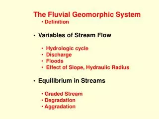
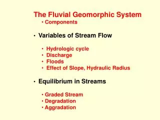
The Fluvial Geomorphic System Components Variables of Stream Flow Hydrologic cycle Discharge Floods Effect of Slope, Hydraulic Radius Equilibrium in Streams Graded Stream Degradation Aggradation. The Fluvial Geomorphic System.

E N D
The Fluvial Geomorphic System • Components • Variables of Stream Flow • Hydrologic cycle • Discharge • Floods • Effect of Slope, Hydraulic Radius • Equilibrium in Streams • Graded Stream • Degradation • Aggradation
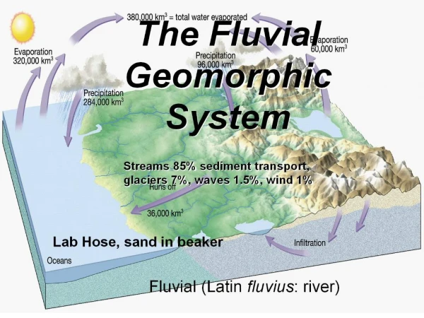
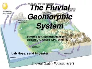
The Fluvial Geomorphic System • How is sediment transported and removed from continents? • (i.e., what mechanisms are most important • in shaping landscapes?) ► Rivers: 85-90% ► Glaciers: 7% ► Groundwater & Waves: 1-2% ► Wind: < 1% ► Volcanoes: < 1%
The fluvial system is comprised of these components: ► Drainage divides, ► Source areas of water and sediment, ► Channels and valleys of the drainage basin (watershed ), ► Depositional Areas
Example watershed--sketch Terminus or drain point
Example watershed—on shaded relief map Terminus or drain point
Hydrologic cycle Water budget/balance: Inputs – Outputs = +/- Storage Inputs? precipitation Outputs? evapotranspiration runoff GW discharge Storage? Soil moisture Flooding aquifer storage
Inputs – Outputs = +/- Storage PCIP - (ET + RO + GW) = ΔS PCIP - ET - RO - GW = ΔS PCIP = ET + RO + GW + ΔS 100% 25-40%
Discharge Cross-sectional area and wetted perimeter d w Area = w x d Wetted perimeter = w + 2d
Discharge d w Cross-sectional area and wetted perimeter 2d 2w Area = 2w x 2d = 4wd Wetted perimeter = 2w + 2(2d) = 2w + 4d
Discharge Area A = wd Area B = 2w x 2d = 4wd Area B / Area A = 4wd / wd = 4 ----------------------------------------------------------- Wetted perimeter A = w + 2d Wetted perimeter B = 2w + 2(2d) = 2w + 4d Wetted perimeter B= 2(w + 2d) Wetted perimeter B / Wetted perimeter A = 2(w + 2d) / (w + 2d) = 2
Discharge d w Cross-sectional area and wetted perimeter • Small increase in wetted perimeter (relative to increase in area) means less frictional resistance, water can flow faster (increased velocity)
Discharge V W D Cross-sectional area and wetted perimeter Result: increased discharge (Q) is caused by increases in width, depth and velocity Q = w x d x v
Discharge Q = w x d x v w = aQb d = cQf v = kQm Q = aQbx cQf x kQm Q = ackQ(b + f+m) a x c x k = 1 b + f + m =1
w = aQb,d = cQf , v = kQm log w = log (a Qb) = log a + b log Q log w = constant + b log Q w = b Q + constant (form of y = mx + b) (plots as line on log-log graph) Discharge
Floods James River in Richmond, Virginia at flood stage, November 1985. Photo by Rick Berquist, used with permission.
Floods Hydrograph: a plot of river level (or discharge) versus time Note equivalence of river elevation (stage) and discharge River Elevation Time Start of rainstorm End of rainstorm
Floods Different watersheds display different hydrograph characteristics small stream larger river in large watershed River Elevation Time
Precipitation Runoff Ground Infiltration Prior to urbanization River Elevation Time Start of rainstorm End of rainstorm
Precipitation Runoff Ground Infiltration Prior to urbanization River Elevation Time Start of rainstorm End of rainstorm
prior to urbanization Precipitation after urbanization Increased Runoff Impervious Ground Little Infiltration River Elevation Time Start of rainstorm End of rainstorm
1993 Mississippi River Flood (500-year flood) Soil Moisture (brighter = wetter) June 6, 1993 July 29, 1993 July 15, 1993 http://www.cgrer.uiowa.edu/research/exhibit_gallery/great_floods/wetness.html
dry soils Precipitation saturated soils Increased Runoff Impervious Ground Little Infiltration River Elevation Time Start of rainstorm End of rainstorm
Floods Constructing a rating curve Note equivalence of stage and discharge
Example rating curve Note that rating curve allows estimation of discharge for extreme floods.
Estimating stage level of past floods— can then use rating curve to estimate discharge
Wayne Co. flood case STEEP VALLEY WALL WATTS HOME WATER LEVEL, 11/12/03 RR TRACKS FLOOD PLAIN ~6-8 ft ~5-7 ft BASE OF DITCH OLD CULVERT ~17 ft ~10-12 ft Normal water level TWELVEPOLE CREEK NOT TO SCALE
Floods • Recurrence interval (RI) is the average number of years between • a flood of a given magnitude. • For example: the 100-year flood is the stage or discharge that occurs • on average every 100 years. • Different for every river. • Data less reliable for larger RI. Why? • RI = (N +1) / m • N = # of years of record , m = rank • Example: If records were kept for 59 years (N=59), and a stage • level of 52 ft was the third highest level (m=3) reached during this • period, then a flood of this magnitude would be categorized as a 20-year • flood (RI = 60/3).
Miss. River, Chester, Il – 1993 Note that the probability of a flood of a given magnitude is 1/RI. Example: In any year, the chance of a100-year flood is 1/100 = 1% The mean annual flood is the average of the maximum annual floods over a period of years. RImean = 2.33
Floods James River in Richmond, Virginia at flood stage, November 1985. Photo by Rick Berquist, used with permission.
Flood Exercise • James River, Richmond VA • Three largest floods recorded from 1935 to present. • 1. June 23, 1972, 28.62 ft (gage height), 313,000 cfs (discharge) • August 21, 1969, 24.95 ft (gage height), 222,000 cfs (discharge) • November 7, 1985, 24.77 ft (gage height), 218,000 cfs (discharge) • From the picture of the river at normal flow, estimate the stage at these conditions. • Calculate RI and probability for each of these flood events
Floods Paleofloods • Causes: dam outbursts, glacial outbursts, extreme precipitation events. • ice dam collapsed during last Ice Age in eastern Washington, emptying • lake about half size of Lake Michigan; floodwaters had Q~752,000,000 cfs. • Provide direct evidence of extreme hydrologic events that may shed light • back to mid-Holocene (~5,000 years) • Flood deposits and flood erosional effects are primary sources of • information about the magnitude and frequency of these extreme events.
Floods Paleofloods Example use of paleoflood records to discern mid- Holocene climates Hirschboeck, 2003
Q = w x d x v Floods Paleoflood “reconstruction” • What is needed to estimate discharge, Q, during a modern flood? • Rating curve allows Q to be estimated from stage • What is needed to estimate discharge during a paleoflood? • flood stage may not be known • If flood stage is known, no rating curve for extreme stage • velocity must be estimated and ancient valley shape must be estimated
Floods Paleoflood “reconstruction” • Methods for estimating stage of paleofloods • depositional: slack-water deposits in tributary valleys, caves, etc. • slack-water deposits formed during sudden velocity decreases following peak discharge • only preserved in protected areas above elevation of modern floods • (“non-exceedance level” • erosional: terrace benches, markings on paleosols, bedrock walls, etc. • vegetation: damaged trees, etc.
Floods Paleofloods Hirschboeck, 2003
d d w Floods Paleoflood “reconstruction” • Methods for estimating velocity of paleofloods • quantitative empirical or theoretical relationships • Chezy formula: uses hydraulic radius and slope to estimate velocity • Use sizes of boulders transported in flood to estimate velocity • Manning equation: uses hydraulic radius and slope to estimate velocity: • v = 1.49/n x R2/3 x S1/2 • n = roughness factor • R = hydraulic radius • S = slope Wetted perimeter (WP) = 2d + w Area (A) = wd R = A / WP = wd / (2d + w)
d d w Relationships among channel shape, velocity, slope and erosional energy • Manning equation: relates hydraulic radius and slope to velocity • v = 1.49/n x R2/3 x S1/2 • n = roughness factor • R = hydraulic radius • S = slope Wetted perimeter (WP) = 2d + w Area (A) = wd R = A / WP = wd / (2d + w)
1 20 2 10 Relationships among channel shape, velocity and erosional energy Wetted perimeter (WP) = 2d + w Area (A) = wd R = A / WP = wd / (2d + w) WP = 14 A = 20 R = 1.4 WP = 22 A = 20 R = 0.9
1 20 2 10 Relationships among channel shape, velocity and erosional energy • What does Manning equation say about flow in these two different • channel shapes if slope and roughness are equal? • v = 1.49/n x R2/3 x S1/2 • n = roughness factor • R = hydraulic radius • S = slope • larger radius means greater velocity. • smaller radius means less velocity. • Tendency of smaller radius to restrict velocity is result of turbulence and friction as water contacts the channel margins. This causes erosion ! WP = 14 A = 20 R = 1.4 WP = 22 A = 20 R = 0.9
1 20 2 10 Relationships among channel shape, velocity, slope and erosional energy Hydraulic shear WP = 14 A = 20 R = 1.4 WP = 22 A = 20 R = 0.9