Download
1 / 37
370 likes | 605 Views
C. E. N. T. E. R. F. O. R. I. N. T. E. G. R. A. T. I. V. E. B. I. O. I. N. F. O. R. M. A. T. I. C. S. V. U. 1-month Practical Course Genome Analysis Evolution and Phylogeny methods Centre for Integrative Bioinformatics VU (IBIVU) Vrije Universiteit Amsterdam

E N D
C E N T E R F O R I N T E G R A T I V E B I O I N F O R M A T I C S V U 1-month Practical Course Genome AnalysisEvolution and Phylogeny methods Centre for Integrative Bioinformatics VU (IBIVU) Vrije Universiteit Amsterdam The Netherlands www.ibivu.cs.vu.nl heringa@cs.vu.nl
Bioinformatics • “Nothing in Biology makes sense except in the light of evolution” (Theodosius Dobzhansky (1900-1975)) • “Nothing in bioinformatics makes sense except in the light of Biology”
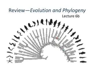
Evolution • Most of bioinformatics is comparative biology • Comparative biology is based upon evolutionary relationships between compared entities • Evolutionary relationships are normally depicted in a phylogenetic tree
Where can phylogeny be used • For example, finding out about orthology versus paralogy • Predicting secondary structure of RNA • Studying host-parasite relationships • Mapping cell-bound receptors onto their binding ligands • Multiple sequence alignment (e.g. Clustal)
Gene conversion • The transfer of DNA sequences between two homologous genes, most often by unequal crossing over during meiosis • Can be a mechanism for mutation if the transfer of material disrupts the coding sequence of the gene or if the transferred material itself contains one or more mutations
Gene conversion • Gene conversion can influence the evolution of gene families, having the capacity to generate both diversity and homogeneity. • Example of a intrachromosomal geneconversion event: • The potential evolutionary significance of gene conversion is directly related to its frequency in the germ line. While meiotic inter- and intrachromosomal gene conversionis frequent in fungal systems, it has hitherto been considered impractical in mammals. However, meiotic gene conversion has recently been measured as a significant recombination process, for example in mice.
DNA evolution • Gene nucleotide substitutions can be synonymous (i.e. not changing the encoded amino acid) or nonsynonymous (i.e. changing the a.a.). • Rates of evolution vary tremendously among protein-codinggenes. Molecular evolutionary studies have revealed an∼1000-fold range of nonsynonymous substitution rates (Liand Graur 1991). • The strength of negative (purifying) selectionis thought to be the most important factor in determiningthe rate of evolution for the protein-coding regions of agene (Kimura 1983; Ohta 1992; Li 1997).
DNA evolution • “Essential” and “nonessential” are classic moleculargenetic designations relating to organismal fitness. • A gene is considered to be essential if a knock-outresults in (conditional) lethality or infertility. • Nonessential genes are those for which knock-outs yieldviable and fertile individuals. • Given the role of purifyingselection in determining evolutionary rates, thegreater levels of purifying selection on essential genes leads to a lower rate of evolution relative to that ofnonessential genes.
Reminder -- Orthology/paralogy Orthologous genes are homologous (corresponding) genes in different species Paralogous genes are homologous genes within the same species (genome)
Orthology/paralogy • Operational definition of orthology: • Bi-directional best hit: • Blast gene A in genome 1 against genome 2: gene B is best hit • Blast gene B against genome 1: if gene A is best hit • A and B are orthologous
Old Dogma – Recapitulation Theory (1866) Ernst Haeckel: “Ontogeny recapitulates phylogeny” Ontogeny is the development of the embryo of a given species; phylogeny is the evolutionary history of a species http://en.wikipedia.org/wiki/Recapitulation_theory Haeckels drawing in support of his theory: For example, the human embryo with gill slits in the neck was believed by Haeckel to not only signify a fishlike ancestor, but it represented a total fishlike stage in development. Gill slits are not the same as gills and are not functional.
Phylogenetic tree (unrooted) human Drosophila internal node fugu mouse leaf OTU – Observed taxonomic unit edge
Phylogenetic tree (unrooted) root human Drosophila internal node fugu mouse leaf OTU – Observed taxonomic unit edge
Phylogenetic tree (rooted) root time edge internal node (ancestor) leaf OTU – Observed taxonomic unit Drosophila human fugu mouse
How to root a tree m f • Outgroup – place root between distant sequence and rest group • Midpoint – place root at midpoint of longest path (sum of branches between any two OTUs) • Gene duplication – place root between paralogous gene copies h D f m h D 1 m f 3 1 2 4 2 3 1 1 1 h 5 D f m h D f- f- h- f- h- f- h- h-
Combinatoric explosion Number of unrooted trees = Number of rooted trees =
Combinatoric explosion # sequences # unrooted # rooted trees trees 2 1 1 3 1 3 4 3 15 5 15 105 6 105 945 7 945 10,395 8 10,395 135,135 9 135,135 2,027,025 10 2,027,025 34,459,425
Tree distances Evolutionary (sequence distance) = sequence dissimilarity 5 human x mouse 6 x fugu 7 3 x Drosophila 14 10 9 x human 1 mouse 2 1 1 fugu 6 Drosophila mouse Drosophila human fugu Note that with evolutionary methods for generating trees you get distances between objects by walking from one to the other.
Phylogeny methods • Distance based – pairwise distances (input is distance matrix) • Parsimony – fewest number of evolutionary events (mutations) – relatively often fails to reconstruct correct phylogeny, but methods have improved recently • Maximum likelihood – L = Pr[Data|Tree] – most flexible class of methods - user-specified evolutionary methods can be used
Distance based --UPGMA Let Ci andCj be two disjoint clusters: 1 di,j = ————————pqdp,q, where p Ci and q Cj |Ci| × |Cj| Ci Cj In words: calculate the average over all pairwise inter-cluster distances
Clustering algorithm: UPGMA • Initialisation: • Fill distance matrix with pairwise distances • Start with N clusters of 1 element each • Iteration: • Merge cluster Ci and Cj for which dij is minimal • Place internal node connecting Ci and Cj at height dij/2 • Delete Ci and Cj (keep internal node) • Termination: • When two clusters i, j remain, place root of tree at height dij/2 d
Ultrametric Distances • A tree T in a metric space (M,d) where d is ultrametric has the following property: there is a way to place a root on T so that for all nodes in M, their distance to the root is the same. Such T is referred to as a uniformmolecular clock tree. • (M,d) is ultrametric if for every set of three elements i,j,k∈M, two of the distances coincide and are greater than or equal to the third one (see next slide). • UPGMA is guaranteed to build correct tree if distances are ultrametric. But it fails if not!
Evolutionary clock speeds Uniform clock: Ultrametric distances lead to identical distances from root to leafs Non-uniform evolutionary clock: leaves have different distances to the root -- an important property is that of additive trees. These are trees where the distance between any pair of leaves is the sum of the lengths of edges connecting them. Such trees obey the so-called 4-point condition (next slide).
Additive trees In additive trees, the distance between any pair of leaves is the sum of lengths of edges connecting them Given a set of additive distances: a unique tree T can be constructed: For all trees: if d is ultrametric ==> d is additive
Distance based --Neighbour-Joining (Saitou and Nei, 1987) • Guaranteed to produce correct tree if distances are additive • May even produce good tree if distances are not additive • Global measure – keeps total branch length minimal • At each step, join two nodes such that distances are minimal (criterion of minimal evolution) • Agglomerative algorithm • Leads to unrooted tree
Neighbour joining y x x x y (c) (a) (b) x x x y y (f) (d) (e) At each step all possible ‘neighbour joinings’ are checked and the one corresponding to the minimal total tree length (calculated by adding all branch lengths) is taken.
Algorithm: Neighbour joining • NJ algorithm in words: • Make star tree with ‘fake’ distances (we need these to be able to calculate total branch length) • Check all n(n-1)/2 possible pairs and join the pair that leads to smallest total branch length. You do this for each pair by calculating the real branch lengths from the pair to the common ancestor node (which is created here – ‘y’ in the preceding slide) and from the latter node to the tree • Select the pair that leads to the smallest total branch length (by adding up real and ‘fake’ distances). Record and then delete the pair and their two branches to the ancestral node, but keep the new ancestral node. The tree is now 1 one node smaller than before. • Go to 2, unless you are done and have a complete tree with all real branch lengths (recorded in preceding step)
Parsimony & Distance parsimony Sequences 1 2 3 4 5 6 7 Drosophila t t a t t a a fugu a a t t t a a mouse a a a a a t a human a a a a a a t Drosophila mouse 1 6 4 5 2 3 7 human fugu distance human x mouse 2 x fugu 4 4 x Drosophila5 5 3 x Drosophila 2 mouse 1 2 1 1 human fugu mouse Drosophila human fugu
Maximum likelihood • If data=alignment, hypothesis = tree, and under a given evolutionary model, maximum likelihood selects the hypothesis (= tree) that maximises the observed data (= alignment). So, you keep alignment constant and vary the trees. • Extremely time consuming method • We also can also test the relative fit to the tree of different models (Huelsenbeck & Rannala, 1997). Now you vary the trees and the models (and keep the alignment constant)
Distance methods: fastest • Clustering criterion using a distance matrix • Distance matrix filled with alignment scores (sequence identity, alignment scores, E-values, etc.) • Cluster criterion
Phylogenetic tree by Distance methods (Clustering) 1 2 3 4 5 Multiple alignment Similarity criterion Similarity matrix Scores 5×5 Phylogenetic tree
Human -KITVVGVGAVGMACAISILMKDLADELALVDVIEDKLKGEMMDLQHGSLFLRTPKIVSGKDYNVTANSKLVIITAGARQ Chicken -KISVVGVGAVGMACAISILMKDLADELTLVDVVEDKLKGEMMDLQHGSLFLKTPKITSGKDYSVTAHSKLVIVTAGARQ Dogfish –KITVVGVGAVGMACAISILMKDLADEVALVDVMEDKLKGEMMDLQHGSLFLHTAKIVSGKDYSVSAGSKLVVITAGARQ Lamprey SKVTIVGVGQVGMAAAISVLLRDLADELALVDVVEDRLKGEMMDLLHGSLFLKTAKIVADKDYSVTAGSRLVVVTAGARQ Barley TKISVIGAGNVGMAIAQTILTQNLADEIALVDALPDKLRGEALDLQHAAAFLPRVRI-SGTDAAVTKNSDLVIVTAGARQ Maizey casei -KVILVGDGAVGSSYAYAMVLQGIAQEIGIVDIFKDKTKGDAIDLSNALPFTSPKKIYSA-EYSDAKDADLVVITAGAPQ Bacillus TKVSVIGAGNVGMAIAQTILTRDLADEIALVDAVPDKLRGEMLDLQHAAAFLPRTRLVSGTDMSVTRGSDLVIVTAGARQ Lacto__ste -RVVVIGAGFVGASYVFALMNQGIADEIVLIDANESKAIGDAMDFNHGKVFAPKPVDIWHGDYDDCRDADLVVICAGANQ Lacto_plant QKVVLVGDGAVGSSYAFAMAQQGIAEEFVIVDVVKDRTKGDALDLEDAQAFTAPKKIYSG-EYSDCKDADLVVITAGAPQ Therma_mari MKIGIVGLGRVGSSTAFALLMKGFAREMVLIDVDKKRAEGDALDLIHGTPFTRRANIYAG-DYADLKGSDVVIVAAGVPQ Bifido -KLAVIGAGAVGSTLAFAAAQRGIAREIVLEDIAKERVEAEVLDMQHGSSFYPTVSIDGSDDPEICRDADMVVITAGPRQ Thermus_aqua MKVGIVGSGFVGSATAYALVLQGVAREVVLVDLDRKLAQAHAEDILHATPFAHPVWVRSGW-YEDLEGARVVIVAAGVAQ Mycoplasma -KIALIGAGNVGNSFLYAAMNQGLASEYGIIDINPDFADGNAFDFEDASASLPFPISVSRYEYKDLKDADFIVITAGRPQ Lactate dehydrogenase multiple alignment Distance Matrix 1 2 3 4 5 6 7 8 9 10 11 12 13 1 Human 0.000 0.112 0.128 0.202 0.378 0.346 0.530 0.551 0.512 0.524 0.528 0.635 0.637 2 Chicken 0.112 0.000 0.155 0.214 0.382 0.348 0.538 0.569 0.516 0.524 0.524 0.631 0.651 3 Dogfish 0.128 0.155 0.000 0.196 0.389 0.337 0.522 0.567 0.516 0.512 0.524 0.600 0.655 4 Lamprey 0.202 0.214 0.196 0.000 0.426 0.356 0.553 0.589 0.544 0.503 0.544 0.616 0.669 5 Barley 0.378 0.382 0.389 0.426 0.000 0.171 0.536 0.565 0.526 0.547 0.516 0.629 0.575 6 Maizey 0.346 0.348 0.337 0.356 0.171 0.000 0.557 0.563 0.538 0.555 0.518 0.643 0.587 7 Lacto_casei 0.530 0.538 0.522 0.553 0.536 0.557 0.000 0.518 0.208 0.445 0.561 0.526 0.501 8 Bacillus_stea 0.551 0.569 0.567 0.589 0.565 0.563 0.518 0.000 0.477 0.536 0.536 0.598 0.495 9 Lacto_plant 0.512 0.516 0.516 0.544 0.526 0.538 0.208 0.477 0.000 0.433 0.489 0.563 0.485 10 Therma_mari 0.524 0.524 0.512 0.503 0.547 0.555 0.445 0.536 0.433 0.000 0.532 0.405 0.598 11 Bifido 0.528 0.524 0.524 0.544 0.516 0.518 0.561 0.536 0.489 0.532 0.000 0.604 0.614 12 Thermus_aqua 0.635 0.631 0.600 0.616 0.629 0.643 0.526 0.598 0.563 0.405 0.604 0.000 0.641 13 Mycoplasma 0.637 0.651 0.655 0.669 0.575 0.587 0.501 0.495 0.485 0.598 0.614 0.641 0.000
How to assess confidence in tree How sure are we about these splits?
How to assess confidence in tree • Bayesian method – time consuming • The Bayesian posterior probabilities (BPP) are assigned to internal branches in consensus tree • Bayesian Markov chain Monte Carlo (MCMC) analytical software such as MrBayes (Huelsenbeck and Ronquist, 2001) and BAMBE (Simon and Larget,1998) is now commonly used • Uses all the data • Distance method – bootstrap: • Select multiple alignment columns with replacement • Recalculate tree • Compare branches with original (target) tree • Repeat 100-1000 times, so calculate 100-1000 different trees • How often is branching (point between 3 nodes) preserved for each internal node? • Uses samples of the data
The Bootstrap 1 2 3 4 5 6 7 8 C C V K V I Y S M A V R L I F S M C L R L L F T 3 4 3 8 6 6 8 6 V K V S I I S I V R V S I I S I L R L T L L T L 5 1 2 3 Original 4 2x 3x 1 1 2 3 Non-supportive Scrambled 5
Phylogeny disclaimer • With all of the phylogenetic methods, you calculate one tree out of very many alternatives. • Only one tree can be correct and depict evolution accurately. • Incorrect trees will often lead to ‘more interesting’ phylogenies, e.g. the whale originated from the fruit fly etc.
Take home messages • Orthology/paralogy • Rooted/unrooted trees • Make sure you know the issues around the UPGMA algorithm and the NJ algorithm • Understand the three basic classes of phylogenetic methods: distance, parsimony and maximum likelihood • Make sure you understand bootstrapping (to asses confidence in tree splits)