Download
1 / 27
270 likes | 343 Views
Explore modeling stochastic circuit behavior in IC technology scaling, focusing on performance probability distribution extraction. The paper introduces proposed algorithms for efficient high-order moment calculations using Point Estimation Method.

E N D
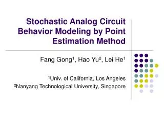
Stochastic Analog Circuit Behavior Modeling by PointEstimation Method Fang Gong1, Hao Yu2, Lei He1 1Univ. of California, Los Angeles 2Nanyang Technological University, Singapore
Outline • Backgrounds • Existing Methods and Limitations • Proposed Algorithms • Experimental Results • Conclusions
90nm 65nm 45nm Shrinking Feature Sizes IC Technology Scaling • Feature size keeps scaling down to 45nm and below • Large process variation lead to circuit failures and yield problem. * Data Source: Dr. Ralf Sommer, DATE 2006, COM BTS DAT DF AMF;
Statistical methods were proposed to address variation problems Focus on performance probability distributionextraction in this work Fixed Value Random Distribution Process Parameters Design Parameters Statistical Problems in IC Technology Parameter Space Mapping? Unknown Distribution Circuit Performance Performance Space How to model the stochastic circuit behavior (performance)?
Leakage Power Distribution • An example ISCAS-85 benchmark circuit: • all threshold voltages (Vth) of MOSFETs have variations that follow Normal distribution. • The leakage power distribution follow lognormal distribution. • It is desired to extract thearbitrary (usually non-normal)distribution of performance exactly. *Courtesy by Fernandes, R.; Vemuri, R.; , ICCD 2009. pp.451-458, 4-7 Oct. 2009
Problem Formulation • Given: random variablesin parameter space • a set of (normal) random variables {ε1, ε2, ε3, ...} to model process variation sources. • Goal: extract the arbitraryprobability distribution of performance f(ε1, ε2, ε3, ...) in performance space. Variable performance process variation mapping Performance Space Parameter Space
Outline • Backgrounds • Existing Methods and Limitations • Proposed Algorithms • Experimental Results • Conclusions
Device variation SPICE Monte Carlo Analysis Performance Domain Parameter Domain Monte Carlo simulation • Monte Carlo simulation is the most straight-forward method. • However, it is highly time-consuming!
f Δx1 Δx2 Response Surface Model (RSM) • Approximate circuit performance (e.g. delay) as an analytical function of all process variations (e.g. VTH, etc ) • Synthesize analytical function of performance as random variations. • Results in a multi-dimensional model fitting problem. • Response surface model can be used to • Estimate performance variability • Identify critical variation sources • Extract worst-case performance corner • Etc.
Flow Chart of APEX* Synthesize analytical function of performance using RSM Calculate moments Calculate the probability distribution function (PDF) of performance based on RSM h(t) can be used to estimate pdf(f) *Xin Li, Jiayong Le, Padmini Gopalakrishnan and Lawrence Pileggi, "Asymptotic probability extraction for non-Normal distributions of circuit performance," IEEE/ACMInternational Conference on Computer-Aided Design (ICCAD), pp. 2-9, 2004.
Limitation of APEX • RSM based method is time-consuming to get the analytical function of performance. • It has exponential complexity with the number of variable parameters n and order of polynomial function q. • e.g., for 10,000 variables, APEX requires 10,000 simulations for linear function, and 100 millions simulations for quadratic function. • RSM based high-order moments calculation has high complexity • the number of terms in fkincreases exponentially with the order of moments.
Step 1: Calculate High Order Moments of Performance Contribution of Our Work APEX Proposed Method • Our contribution: • We do NOT need to use analytical formula in RSM; • Calculate high-order moments efficiently using Point Estimation Method; Find analytical function of performance using RSM A few samplings at selected points. Calculate high order moments Calculate moments by Point Estimation Method Step 2: Extract the PDF of performance
Outline • Backgrounds • Existing Methods and Limitations • Proposed Algorithms • Experimental Results • Conclusions
Moments via Point Estimation • Point Estimation: approximate high order moments with a weighted sum of sampling values of f(x). • are estimating points of random variable. • Pj are corresponding weights. • k-th moment of f(x) can be estimated with • Existing work in mechanical area* only provide empirical analytical formulae for xj and Pj for first four moments. f(x2) f(x1) f(x3) PDF x1 x2 x3 Question – how can we accurately and efficiently calculate the higher order moments of f(x)? * Y.-G. Zhao and T. Ono, "New point estimation for probability moments," Journal of Engineering Mechanics, vol. 126, no. 4, pp. 433-436, 2000.
Calculate moments of performance • Theorem in Probability: assume x and f(x) are both continuous random variables, then: • Flow Chart to calculate high order moments of performance: Step 5: extract performance distribution pdf(f) pdf(x) of parameters is known Step 1: calculate moments of parameters Step 4: calculate moments of performance Step 2: calculate the estimating points xjand weights Pj Step 3: run simulation at estimating points xj and get performance samplings f(xj) Step 2 is the most important step in this process.
Estimating Points xj and Weights Pj • With moment matching method,and Pj can be calculated by • can be calculated exactly with pdf(x). • Assume residues aj= Pj and poles bj= • system matrix is well-structured (Vandermonde matrix); • nonlinear system can solved with deterministic method.
Extension to Multiple Parameters • Model moments with multiple parameters as a linear combination of moments with single parameter. • f(x1,x2,…,xn) is the function with multiple parameters. • f(xi) is the function where xi is the single parameter. • gi is the weight for moments of f(xi) • c is a scaling constant.
Error Estimation • We use approximation with q+1 moments as the exact value, when investigating PDF extracted with q moments. • When moments decrease progressively • Other cases can be handled after shift (f<0),reciprocal (f>1) or scaling operations of performance merits. 0 < f < 1 Magnitude of Moment (normalized) Order of Moment
Outline • Backgrounds • Existing Methods and Limitations • Proposed Algorithms • Experimental Results • Conclusions
(1) Validate Accuracy: Settings MMC+APEXRun Monte Carlo PEMPoint Estimation • To validate accuracy, we compare following methods: • Monte Carlo simulation. • run tons of SPICE simulations to get performance distribution. • PEM: point estimation based method (proposed in this work) • calculate high order moments with point estimation. • MMC+APEX: • obtain the high order moments from Monte Carlo simulation. • perform APEX analysis flow with these high-order moments. Calculate time moments Match with the time moment of a LTI system
6-T SRAM Cell • Study the discharge behavior in BL_B node during reading operation. • Consider threshold voltage of all MOSFETs as independent Gaussian variables with 30% perturbation from nominal values. • Performance merit is the voltage difference between BL and BL_B nodes.
PDF 0 Accuracy Comparison • Variations in threshold voltage lead to deviations on discharge behavior • Investigate distribution of node voltage at certain time-step. • Monte Carlo simulation is used as baseline. • Both APEX and PEM can provide high accuracy when compared with MC simulation. Probability of Occurrence (Normalized) MC results Voltage (volt)
(2)Validate Efficiency: PEM vs. MC • For 6-T SRAM Cell, Monte Carlo methods requires 3000 times simulations to achieve an accuracy of 0.1%. • Point Estimation based Method (PEM) needs only 25 times simulations, and achieve up to 119X speedup over MC with the similar accuracy.
Compare Efficiency: PEM vs. APEX • To compare with APEX: • One Operational Amplifier under a commercial 65nm CMOS process. • Each transistor needs 10 independent variables to model the random variation*. • We compare the efficiency between PEM and APEX by the required number of simulations. • Linear vs. Exponential Complexity: • PEM: alinear function of number of sampling point and random variables. • APEX: anexponential function of polynomial order and number of variables. * X. Li and H. Liu, “Statistical regression for efficient high-dimensional modeling of analog and mixed-signal performance variations," in Proc. ACM/IEEE Design Automation Conf. (DAC), pp. 38-43, 2008.
~124X Polynomial Order in RSM Operational Amplifier • A two-stage operational amplifier • complexity in APEX increases exponentially with polynomial orders and number of variables. • PEM has linear complexity with the number of variables. Operational Amplifier with 500 variables Quadratic polynomial case ~124X The Y-axis in both figures has log scale!
Conclusion • Studied stochastic analog circuit behavior modeling under process variations • Leverage the Point Estimation Method (PEM) to estimate the high order moments of circuit behavior systematicallyand efficiently. • Compared with exponential complexity in APEX, proposed method can achieve linear complexity of random variables.
Thank you! ACM International Symposium on Physical Design 2011 Fang Gong, Hao Yu and Lei He